Spectral Synthesis¶

This tutorial shows how compute transmission, emission, or eclipse spectra with Pyrat Bay.

Configuration File
System parameters
Stellar Spectrum
Spectrum sampling
Observations
Atmosphere Model
Cross sections
Fitting parameters
Examples

Configuration File¶

To compute spectra, use a configuration file with the runmode key set to spectrum. Spectrum runs also require a logfile key, which sets the name of the output log and spectrum files.

Observing Geometry

The rt_path key sets the radiative-transfer scheme and observing geometry to use. These are the options:

Observing geometry	`rt_path`	Output spectrum	Comments
Transmission	`transit`	(\(R_{\rm p}\)/\(R_{\rm s}\))²	Transmission spectrum

Eclipse	`eclipse`	\(F_{\rm p}\)/\(F_{\rm s}\)	Occultation spectrum
Eclipse	`eclipse_two_stream`	\(F_{\rm p}\)/\(F_{\rm s}\)	Appendix B of [Heng2014]

Emission	`emission`	\(F_{\rm p}\) (erg s⁻¹ cm⁻² cm)	Flux at the planet’s surface
Emission	`emission_two_stream`	\(F_{\rm p}\) (erg s⁻¹ cm⁻² cm)	Appendix B of [Heng2014]
Emission	`f_lambda`	\(F_{\rm p}\) (W m⁻² μm⁻¹)	Flux measured at Earth

Here is a sample configuration file to compute a transmission spectrum:

File spectral_synthesis_transmission.cfg¶

[pyrat]

# Pyrat Bay run mode [tli atmosphere spectrum radeq opacity retrieval]
runmode = spectrum

# Output files
logfile = transmission_spectrum_tutorial.log

# Radiative-transer observing geometry, select from: [transit emission]
rt_path = transit

# Wavelength sampling:
wl_low  = 0.3 um
wl_high = 5.0 um

# System parameters:
rstar = 1.27 rsun
tstar = 5800.0
smaxis = 0.045 au
mplanet = 0.6 mjup
rplanet = 1.0 rjup
# Reference pressure level at rplanet:
refpressure = 0.1 bar

# Atmospheric model:
ptop = 1.0e-8 bar
pbottom = 100.0 bar
nlayers = 81

# Temperature profile [isothermal guillot madhu]
tmodel = isothermal
tpars = 850.0

# Chemistry model [free equilibrium]
chemistry = free
species =       H2    He   Na  H2O  CH4   CO  CO2  NH3  HCN   N2
uniform_vmr = 0.85 0.149 5e-6 2e-3 1e-4 5e-4 1e-6 1e-5 1e-9 2e-4

# Radius-profile model [hydro_m hydro_g]
radmodel = hydro_m


# Line-sampled cross sections
sampled_cross_sec =
    cross_section_0.15-33.0um_0200-5000K_R025K_H2O_exomol_pokazatel.npz

# Continuum cross-section files:
continuum_cross_sec =
    {ROOT}/pyratbay/data/CIA/CIA_Borysow_H2H2_0060-7000K_0.6-500um.dat
    {ROOT}/pyratbay/data/CIA/CIA_Borysow_H2He_0050-3000K_0.3-030um.dat

# Alkali models, select from: [sodium_vdw potassium_vdw]
alkali = sodium_vdw

# Rayleigh models, select from: [rayleigh_H rayleigh_He rayleigh_H2]
rayleigh =
    rayleigh_H2
    rayleigh_He

# Cloud models, select from: [lecavelier deck ccsgray]
clouds =
    deck       -0.5
    lecavelier  0.0 -4.0

# Verbosity level (<0:errors, 0:warnings, 1:headlines, 2:details, 3:debug):
verb = 2

# If defined, plot x-axis in log scale and set ticks at logxticks locations:
logxticks = 0.3 0.5 0.7 1.0 2.0 3.0 5.0

The output spectrum can be set with the specfile key, otherwise it is taken from the logfile name (replacing the .log file extension with .dat)

System parameters¶

The system parameters have multiple uses.

Hill radius¶

The mstar, mplanet, and smaxis keys set the stellar mass, planetary mass, and orbital semi-major axis. If these keys are set in the configuration file, the code will compute the planetary Hill radius (\(R_{\rm H} = a \sqrt[3]{M_{\rm p}/3M_{\rm s}}\)). In such case, Pyrat Bay will neglect atmospheric layers at altitudes larger than \(R_{\rm H}\), since they should not be gravitationally bound to the planet.

Radius ratio¶

To compute eclipse depths from the emission spectra (\(F_{\rm p}\)), the user needs to set the rstar and rplanet keys, which define the stellar and planetary radius. The eclipse depths can then be computed as:

\[{\rm Eclipse\ depth} = \frac{F_{\rm p}}{F_{\rm s}} \left(\frac{R_{\rm p}}{R_{\rm s}}\right)^2\]

The tstar key sets the stellar effective temperature, which can be used to define a stellar blackbody spectrum (\(F_{\rm s}\), see starspec).

Stellar Spectrum¶

The stellar spectrum is required to compute eclipse depths as the planet-to-star flux spectrum (for transit calculations, a stellar spectrum is not required). Pyrat Bay provides several options to set a stellar spectrum.

Custom spectrum

Users can use their own custom stellar spectra via the starspec argument. This must point to a plain file file containing a spectrum in two columns: the first column has the wavelength array in microns, the second column has the flux spectrum in erg s^-1 cm^-2 cm units.

# Custom stellar spectrum file
starspec = inputs/WASP18_spectrum.dat

Kurucz model

Users can use a Kurucz stellar model [Castelli2003] via the kurucz argument of the configuration file, pointing to a Kurucz model. These models can be downloaded from this link. The code selects the correct Kurucz model based on the stellar temperature and surface gravity values:

# Kurucz stellar spectrum
tstar = 5700
log_gstar = 4.5
kurucz = inputs/fp00k2odfnew.pck

Black body

By defining the stellar effective temperature tstar, the code will adopt a blackbody spectrum for the star (unless the starspec or kurucz arguments have been set).

# Stellar effective temperature (K)
tstar = 5700

Atmosphere Model¶

There are four main atmospheric properties to consider (computed in this order): the pressure profile, the temperature, the volume mixing ratios (VMRs), and the radius profile.

These properties can (a) be read from an input file (atmfile), (b) be computed from parametric models, or (c) be calculated from a mix of them. The rules are simple:

if there is an input atmosphere file, read properties from file
if a model and its parameters are defined, the property will be calculculated from the model (overwritting a )

atmospheric file

The atmfile key sets the input atmospheric model from which to compute the spectrum. If the file pointed by atmfile does not exist, the codel will attempt to produce it (provided all necessary input parameters are set in the configuration file). The atmospheric model can be produced with Pyrat Bay or be a custom input from the user.

# Input atmospheric profile
atmfile = wasp80b_custom_profile.atm

atmospheric models

See these sections to compute atmospheric profiles from models:

combined file and models

TBD

Spectrum sampling¶

The wl_low and wl_high keys set the wavelength boundaries for the output spectrum (values must contain units; otherwise, set the units with the wlunits key).

The wnstep sets the sampling rate in cm^-1. Note that this will be the output sampling rate. Internally, Pyrat Bay must compute line profiles at a higher resolution to ensure not to undersample the line profiles. The wnosamp key (an integer) sets the oversampling factor of the high-resolution sampling relative to wnstep (that is, the high-resolution sampling rate is wnstep/wnosamp). Typical values for the optical/IR are wnstep = 1.0 and wnosamp = 2000.

Alternatively, the user can request a constant-resolution output by setting the resolution key (where the resolution is \(R=\lambda/\Delta\lambda\)).

Cross sections¶

See the following sections for available cross sections:

Flux dilution factor¶

Set the f_dilution argument to set an flux dilution factor [Taylor2020], with values between 0–1, which compensates for emission from an inhomogeneous atmosphere. The dilution factor represents the fractional area of the hottest region on the planet (assuming that the colder regions flux is negligible in comparison).

# Flux dilution factor, value between [0--1]:
f_dilution = 0.85

Observations¶

Use the data and uncert keys to set values for observed transit- or eclipse-depth values and their uncertainties, respectively. Logically, you want to set data values corresponding to the filters pass-bands.

Use the dunits key to specify the units of the data and uncert values (default: dunits = none). Typical values are: ‘none’, ‘percent’, or ‘ppm’ (see Units section).

Note

Note that the filters, data, and uncert keys are not strictly required for a spectrum run, but they will allow the code to plot these information if requested (see [link to plots]).

Filter Pass-bands¶

Use the filters key to set the path to instrument filter pass-bands (see [link to formats?]). These can be used to compute band-integrated values for the transmission or eclipse-depth spectra.

Fitting parameters¶

Number of CPUs¶

The ncpu key sets the number of CPUs to use when computing LBL opacities or when running retrievals (default: ncpu = 1).

Verbosity¶

The verb key sets the screen-output and logfile verbosity level. Higher verb values will display increasingly levels of detail according to the following table:

`verb`	Screen Outputs
<0	Errors
0	Warnings
1	Headlines
2	Details
3	Debug

Plane-parallel Hemispheric Integration¶

For eclipse geometry, the code computes the emergent intensity under the plane-parallel approximation, and then it integrates (sums) intensity spectra at different angles with respect to the normal to model the emitted flux spectrum. The raygrid sets the angles (in degrees) where to evaluate these intensities (default: raygrid = 0 20 40 60 80). The user can set custom values for these angles as long as: (1) the first value is zero (normal to the planet’s ‘surface’), (2) they lie in the [0,90) range, and (3) they are increasing order.

Alternatively, the user can set the quadrature key to perform a Gaussian-quadrature integration, where the quadrature value sets number of Gaussian-quadrature points (in which case, raygrid will be ignored).

Examples¶

Note

Before running this example, make sure that you have generated the TLI file from the tli_tutorial_example, generated the atmospheric profiles from the abundance_tutorial_example, and download the configuration file shown above, e.g., with these shell commands:

tutorial_path=https://raw.githubusercontent.com/pcubillos/pyratbay/master/examples/tutorial
wget https://zenodo.org/records/16965391/files/cross_section_0.15-33.0um_0200-5000K_R025K_H2O_exomol_pokazatel.npz

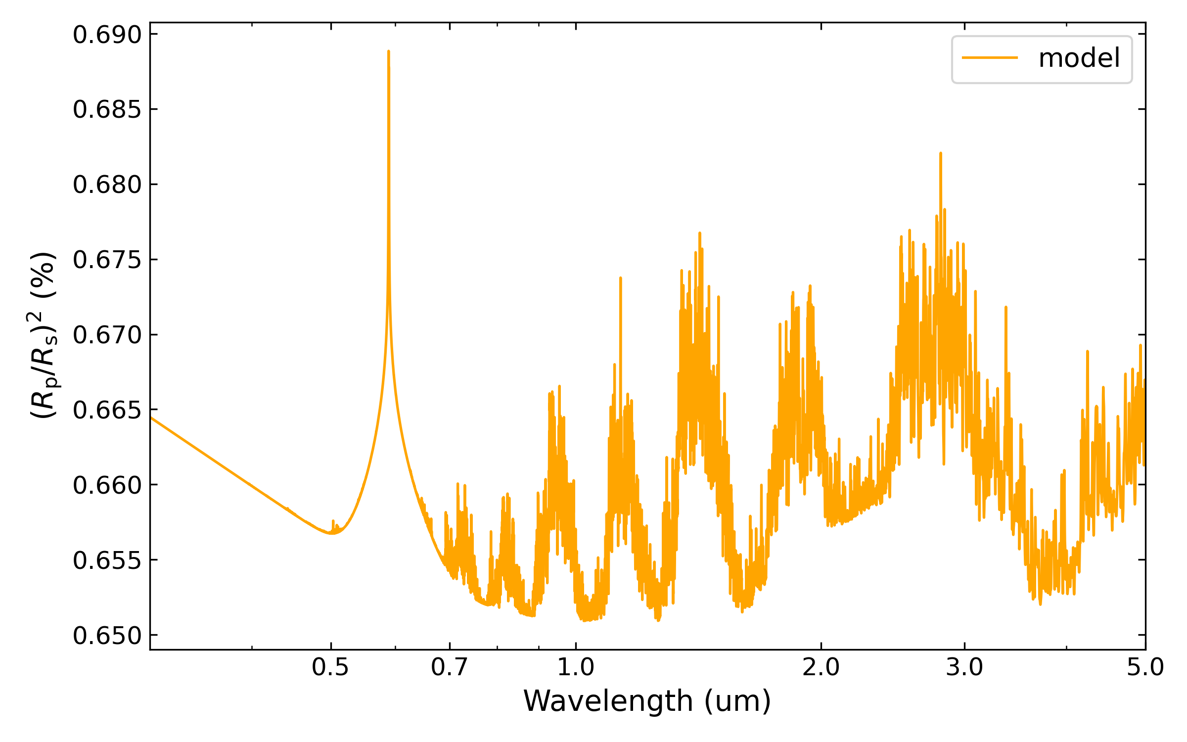
In an interactive run, a spectrum run returns a ‘pyrat’ object that contains all input, intermediate, and output variables used to compute the spectrum. The following Python script computes and plots a transmission spectrum using the configuration file found at the top of this tutorial:

import matplotlib.pyplot as plt
plt.ion()

import pyratbay as pb
import pyratbay.constants as pc

pyrat = pb.run('spectrum_transmission.cfg')

# Plot the resulting spectrum:
wl = 1.0 / (pyrat.spec.wn*pc.um)
depth = pyrat.spec.spectrum / pc.percent
wl_ticks = [0.3, 0.5, 0.7, 1.0, 2.0, 3.0, 5.0]

plt.figure(-3, (7,4))
plt.clf()
ax = plt.subplot(111)
plt.semilogx(wl, depth, "-", color='orange', lw=1.0)
ax.get_xaxis().set_major_formatter(matplotlib.ticker.ScalarFormatter())
ax.set_xticks(wl_ticks)
plt.xlim(0.3, 5.0)
plt.ylabel("Transit depth (Rp/Rs)$^2$ (%)")
plt.xlabel("Wavelength (um)")

# Or, alternatively:
ax = pyrat.plot_spectrum()

And the results should look like this:

_images/pyrat_transmission-spectrum_tutorial.png

Note

Note that although the user can define most input units, nearly all variables are stored in CGS units in the ‘pyrat’ object.

The ‘pyrat’ object is modular, and implements several convenience methods to plot and display its content, as in the following example:

# pyrat object's string representation:
print(pyrat)

# String representation of the spectral variables:
print(pyrat.spec)