Eclipse retrieval: WASP-18b SOSS
This tutorial shows how perform an atmospheric retrieval of the secondary-eclipse spectra of WASP-18b, constrained by the JWST/SOSS observations. We will replicate the analysis presented in [Deline2025], that is, a retrieval of:
the combined JWST, Spitzer, TESS, and CHEOPS observations
1D atmosphere assuming thermochemical-equilibrium VMRs
a Madhu temperature profile, T(p)
a Rayleigh opacity model
a gray, patchy cloud-deck model
We can break the analysis into the following steps:
Setup
For the setup we will need three ingredients:
A configuration file to define the system parameters, atmospheric model, posterior sampling, etc.
An observation file defining the data points: depths, uncertainties, and bin wavelengths
Cross-section files for the atmospheric species
Lets start with the required input files, and then go over the configuration file.
Observation file
Pyrat Bay observation files tell the code what data is being fit.
These are a plain text files containing the transit depth,
uncertainty, and the band (which can be either a tophat or a broadband
passband). There is always one data point per row.
Below you can find an extract of the WASP-18b eclipse data. Click the link to see/download the entire file. Altenatively, you can see the script to make observation files in the right format.
Here’s the observation file containing the CHEOPS, TESS, JWST, and Spitzer data.
Note in the header that comments are allowed, and there are two special flags that let users define the depth units and where the data starts.
Important to note is that:
the first two columns provide the eclipse depth and uncertainties (in the units specified by
@DEPTH_UNITS)the JWST data is modeled as narrow tophat passbands, defined by: the central wavelength, the bin half-width, and (optional) a name for the instrument
the CHEOPS, TESS, and Spitzer data come from broad-band photometry. These we specify as paths to plain files that tabulate the wavelength and response of the band.
Pyrat Bayprovides the passbands for these instruments, indicated by the{FILTERS}path, for other bands one should type the path to the file.
# Passband are either:
# (1) a path to a filter file or
# (2) a tophat defined by a central wavelength, half-width, and a (optional) name

# Comment lines (like this one) and blank lines are ignored,
# central-wavelength and half-width units are always microns

# @DEPTH_UNITS sets the depth and uncert units (e.g., none, percent, ppt, ppm)

@DEPTH_UNITS
ppm

# depth    depth_err   wl         half_width  instrument
@DATA
  357.0     14.0       {FILTERS}/CHEOPS.dat
  357.0     14.0       {FILTERS}/TESS.dat
  486.2     77.2       0.85432    0.00221     NIRISS
  498.7     80.9       0.85918    0.00265     NIRISS
  559.5     78.9       0.86405    0.00221     NIRISS
  520.9     67.3       0.86892    0.00266     NIRISS
  596.9     69.9       0.87381    0.00222     NIRISS
TBD
We will constrain this retrieval to the JWST, Spitzer, CHEOPS, and TESS emission observations. So we need to collect that data. For the JWST spectroscopic observations we will use the NAMELESS spectral reduction (available on Zenodo https://zenodo.org/records/7907569), which we will model as a series of top-hat narrow passbands.
The CHEOPS [Deline2025], TESS [Coulombe2023], and Spitzer [Sheppard2017] observations consist of broad photometric passbands. For these we will use the passband filter files.
Pyrat Bay contains all of this information into an observation
file input. These scripts below show how to create observation
files for (1) the JWST observations, and (2) all photometric and
spectroscopic observations combined.
# Save JWST data
import numpy as np
import pyratbay.io as io

jwst_data = np.loadtxt('NAMELESS_W18b_spectrum.txt', unpack=True)
jwst_wl, jwst_depths, jwst_depth_uncerts, jwst_half_widths = jwst_data
njwst = len(jwst_wl)

# Save JWST data:
obs_file = 'obs_wasp18b_emission_jwst.dat'
jwst_inst_names = ['NIRISS' for _ in jwst_wl]
io.write_observations(
    obs_file,
    jwst_inst_names,
    jwst_wl, jwst_half_widths,
    jwst_depths, jwst_depth_uncerts, depth_units='ppm',
)


# Save JWST + Spitzer + CHEOPS + TESS data:
sheppard2017_spitzer = [2973, 3858, 3700, 4100]
sheppard2017_spitzer_uncerts = [70.0, 113, 300, 200]

coulombe2023_tess = 357.0
coulombe2023_tess_uncert = 14.0

ndata = 2 + njwst + 4
depths = np.zeros(ndata)
depth_uncerts = np.zeros(ndata)

depths[0] = coulombe2023_tess
depths[1] = coulombe2023_tess
depths[2:2+njwst] = jwst_depths
depths[-4:] = sheppard2017_spitzer

depth_uncerts[0] = coulombe2023_tess_uncert
depth_uncerts[1] = coulombe2023_tess_uncert
depth_uncerts[2:2+njwst] = jwst_depth_uncerts
depth_uncerts[-4:] = sheppard2017_spitzer_uncerts

# Leaving the wavelenght values at zero signals to use the instrument
# name as a path to a passband file (for broadband photometry)
wl = np.zeros(ndata)
half_widths = np.zeros(ndata)
wl[2:2+njwst] = jwst_wl
half_widths[2:2+njwst] = jwst_half_widths

spitzer_inst_names = [
    f'{{ROOT}}/pyratbay/data/filters/spitzer_irac{i+1}_sa.dat'
    for i in range(4)
]
inst_names = [
    'CHEOPS.dat',
    'TESS.dat',
]
inst_names += jwst_inst_names + spitzer_inst_names

obs_file = 'obs_wasp18b_emission_all.dat'
io.write_observations(
    obs_file,
    inst_names,
    wl, half_widths,
    depths, depth_uncerts, depth_units='ppm',
)
Cross sections
Following the analysis of [Deline2025], we will include line-sampled cross sections for these molecules: H₂O, CO, CO₂, CH₄, TiO, VO, HCN, NH₃, and C₂H₂. Here we will work with the latests opacity sources for these species from ExoMol and HITEMP.
The current recommendation for sampled cross sections for JWST retrievals is to adopt a resolution \(R>20.000\). So, here we will use a cross section grid at \(R=25.000\), sampling from \(0.35-10.5\) μm in wavelength (to cover the spectral range of the data), from \(500-4000\) K in temperature, and from \(100-1.0^{-9}\) bar in pressure.
Now, beware that cross section files have many assumptions baked into them. In addition, one might need to adjust the ranges or sampling resolution of the grid for specific project. Thus, below there are two options, (a) download and use already made the cross-section files (b) compute your own cross sections starting from the line-list files (where you can customize at will).
The Zenodo repository doi.org/10.5281/zenodo.16965391 contains the cross-section files that we will use for this JWST atmospheric retrieval. See the list below for direct links to the files for each molecule.
These cross sections have been computed assuming an H₂/He-dominated atmosphere, and terrestrial isotopic ratios. The lines have Voigt profiles with a wing cut-off at 300 HWHM and at 25 cm-1. The grids sampling are:
Wavelength: \(0.15-33\) μm, at a constant resolution of \(R=25.000\)
Temperature: \(200-5000\) K, with \(\Delta T = 150\) K
Pressure: \(1.0^{-9}-1.0^{3}\) bar, equally sampled in log(p) with 4 samples per dex.
Species (source) |
References |
|---|---|
H2O (exomol, pokazatel) |
|
CO (HITEMP, li) |
|
CO2 (ames, ai3000k) |
|
CH4 (exomol, mm) |
|
TiO (exomol, toto) |
|
VO (exomol, hyvo) |
|
HCN (exomol, harris larner) |
|
NH3 (exomol, coyute) |
|
C2H2 (exomol, acety) |
Note
If you want to see the source script or need to customize the cross sections (e.g., broader temperature ranges, finer resolution, different line profiles), follow the steps in the ‘Compute cross sections’ tab.
TBD
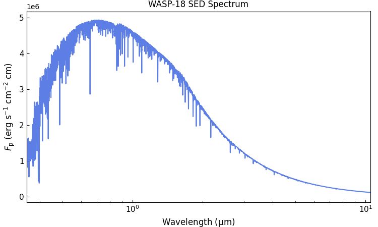
Stellar SED spectrum
The stellar SED is required to calculate the planet-to-star flux
ratio. Here we will use a stellar SED for WASP-18 from the PHOENIX
models [Husser2013], which we will get using the Gen TSO
package. If you haven’t already, install this package with this
shell command:
pip install gen_tso
Now, we can create the stellar SED spectrum with this Python script:
import gen_tso.pandeia_io as pandeia
import pyratbay.constants as pc
import pyratbay.spectrum as ps
import matplotlib.pyplot as plt


# Use the Gen TSO package to get a PHOENIX SED model for WASP-18 (teff=6430.0, logg=4.31)
# Closest SED to WASP-18 is an F5V model (Teff=6500K, logg=4.0)
scene = pandeia.make_scene(
    sed_type='phoenix',
    sed_model='f5v',
)
sed_wl, flux = pandeia.extract_sed(scene, wl_range=(0.35,12.0))
# Convert flux from mJy to erg s-1 cm-2 cm-1
sed_flux = flux * pc.c / 1e26

# Lower the resolution to something closer to NIRISS
bin_wl = ps.constant_resolution_spectrum(0.35, 12.0, resolution=1500.0)
bin_sed_flux = ps.bin_spectrum(bin_wl, sed_wl, sed_flux, gaps='interpolate')

# Save to file
starspec_file = 'phoenix_F5V_6500K_WASP18.dat'
io.write_spectrum(
    bin_wl,
    bin_sed_flux,
    starspec_file,
    type='emission',
)

# Take a look
plt.figure(0, (7.5,4.5))
plt.clf()
plt.subplots_adjust(0.07, 0.11, 0.98, 0.95)
ax = plt.subplot(111)
ax.plot(bin_wl, bin_sed_flux, color='royalblue', alpha=0.85)
ax.set_title('WASP-18 SED Spectrum')
ax.set_xscale('log')
ax.set_xlim(0.35, 10.5)
ax.set_xlabel(r'Wavelength ($\mathrm{\mu}$m)', fontsize=12)
ax.set_ylabel(r'$F_{\rm p}$ (erg s$^{-1}$ cm$^{-2}$ cm)', fontsize=12)
ax.tick_params(direction='in', which='both', labelsize=11)
Configuration file
Lastly, the configuration file will put together the inputs, define the atmospheric model, and configure the retrieval options. Here below is the file we will use for the JWST observation of WASP-39b.
Click here to show/hide: wasp18b_retrieval_eclipse_jwst.cfg
[pyrat]

# Pyrat Bay run mode [tli atmosphere spectrum radeq opacity retrieval]
runmode = retrieval

# Output log and spectrum file names:
logfile = ret_wasp18b_all/WASP18b_eclipse_all.log

# Verbosity level [1--3]:
verb = 2

# Observing geometry, select between: [transit eclipse emission]
rt_path = eclipse

# The observations
dunits = ppm
obsfile = inputs/obs_wasp18b_eclipse_all.dat

# Wavelength sampling
wl_low  = 0.35 um
wl_high = 10.5 um


# System parameters
rstar = 1.23 rsun
mstar = 1.27 msun
tstar = 6435.0

rplanet = 1.165 rjup
mplanet = 10.38 mjup
smaxis = 0.020 au
refpressure = 0.1 bar

# Stellar model
starspec = inputs/phoenix_F5V_6500K_WASP18.dat


# Atmospheric model:
nlayers = 81
ptop = 1e-9 bar
pbottom = 1e2 bar

# Temperature-profile model [isothermal guillot madhu]
tmodel = madhu
#tpars = -3.0 -1.25 1.75 1.0 0.3 2850.0

# Atmospheric composition:
chemistry = equilibrium
species =
    H  He  C  O  N  Na  K  S  Si  Fe  Ti  V
    H2  H2O  CH4  CO  CO2  HCN  NH3  N2  OH  C2H2  C2H4
    S2  SH  SiO  H2S  SO2  SO  TiO  VO  TiO2  VO2
    e-  H-  H+  H2+  He+  Na-  Na+  K-  K+  Fe+  Ti+  V+

# Radius profile model (hydrostatic equilibrium)
radmodel = hydro_m


# Line-sampled cross sections
sampled_cross_sec =
    inputs/cross_section_0.15-33.0um_0200-5000K_R025K_H2O_exomol_pokazatel.npz
    inputs/cross_section_0.15-33.0um_0200-5000K_R025K_CO_hitemp_2019.npz
    inputs/cross_section_0.15-33.0um_0200-5000K_R025K_CO2_ames_ai3000k.npz
    inputs/cross_section_0.15-33.0um_0200-5000K_R025K_TiO_exomol_toto.npz
    inputs/cross_section_0.15-33.0um_0200-5000K_R025K_VO_exomol_hyvo.npz
    inputs/cross_section_0.15-33.0um_0200-5000K_R025K_HCN_exomol_harris_larner.npz
    inputs/cross_section_0.15-33.0um_0200-5000K_R025K_C2H2_exomol_acety.npz
    inputs/cross_section_0.15-33.0um_0200-5000K_R025K_NH3_exomol_coyute.npz
    inputs/cross_section_0.15-33.0um_0200-5000K_R025K_CH4_exomol_mm.npz

# Continuum cross sections
continuum_cross_sec =
    {ROOT}/pyratbay/data/CIA/CIA_Borysow_H2H2_0060-7000K_0.6-500um.dat
    {ROOT}/pyratbay/data/CIA/CIA_Borysow_H2He_0050-7000K_0.5-031um.dat

# Alkali opacity, select from: [sodium_vdw potassium_vdw]
alkali =
    sodium_vdw
    potassium_vdw

# Rayleigh models, select from: [rayleigh_H rayleigh_He rayleigh_H2]
rayleigh =
    rayleigh_H2
    rayleigh_H
    rayleigh_He

# H- continuum opacity
h_ion = h_ion_john1988

# VMR parameters (equilibrium-chemistry)
vmr_vars =
    [M/H]
    [C/H]
    [O/H]

retrieval_params =
# Param_name    value   pmin    pmax   step   prior  prior_sigma
    log_p1      -3.0    -9.0     2.0   0.3
    log_p2      -1.25   -9.0     2.0   0.3
    log_p3       1.75   -9.0     2.0   0.3
    a1           1.00    0.2     2.0   0.02
    a2           0.30    0.2     2.0   0.02
    T0         2850.0  500.0  4000.0   30.0
    [M/H]       1.50    -2.0     2.5   0.1
    [C/H]       0.5     -2.0     2.5   0.1
    [O/H]       0.0     -2.0     2.5   0.1

# Retrieval setup
sampler = multinest
nlive = 1500
resume = True
theme = orange
data_color = black
post_processing = True

# Retrieval temperature boundaries:
tlow  =  500
thigh = 4000

# If set, plot wavelength axes in log-scale, using these tick labels:
wl_ticks = 0.5 0.7 1.0 1.4 2.0 3.0 5.0 8.0
Lets break this down:
# Pyrat Bay run mode [tli atmosphere spectrum radeq opacity retrieval]
runmode = retrieval

# Output log and spectrum file names:
logfile = ret_wasp18b_all/WASP18b_eclipse_all.log

# Verbosity level [1--3]:
verb = 2
This first section defines what we want to run. runmode
indicates that we want a retrieval. logfile sets the path to
the output files. Note that logfile can contain a folder,
which will be created if needed. Finally, verb sets the
screen-output verbosity.
# Observing geometry, select between: [transit eclipse emission]
rt_path = eclipse

# The observations
dunits = ppm
obsfile = inputs/obs_wasp18b_eclipse_all.dat

# Wavelength sampling
wl_low  = 0.35 um
wl_high = 10.5 um
Here we define the observing path of the observation (in this case we have a secondary eclipse), the path to the observation file discussed above (and the desired output units for plots)
wl_low and wl_high set the and the spectral range to model.
Note that the wavelenght sampling is partly set by the
line-sampled opacity files (resolution and maximum wavelength
coverage). One can trim the wavelength ranges (as shown here) to
extract only the region covered by the observations. One can
also lower the resolution via a wl_thinning = n parameter,
which will take every n-th sample of the opacity files (with
n an integer).
# System parameters
rstar = 1.23 rsun
mstar = 1.27 msun
tstar = 6435.0

rplanet = 1.165 rjup
mplanet = 10.38 mjup
smaxis = 0.020 au
refpressure = 0.1 bar

# Stellar model
starspec = inputs/phoenix_F5V_6500K_WASP18.dat
And this section defines the system parameters. For an eclipse run, the relevant properties will be the stellar radius and SED, as well as the planetary mass and radius.
Note that this rplanet value is the reference altitute
situated at the refpressure pressure (this is the constrain
to compute the layer’s \(r(p)\) profile under hydrostatic
equilibrium). Also note that refpressure does not need to be
at one of the sampled layers (it can be anywhere in between the
atmosphere pressure range).
starspec defines the stellar SED: \(F_{\rm
star}(\lambda)\). This is a plain-text file with two columns: the
wavelength (μm) and the surface flux (erg s-1 cm-2 cm). The
eclipse depth is ultimately computed as:
with the rstar and rplanet parameters defining the stellar
and planet radii.
# Atmospheric model:
nlayers = 81
ptop = 1e-9 bar
pbottom = 1e2 bar

# Temperature-profile model [isothermal guillot madhu]
tmodel = madhu
#tpars = -3.0 -1.25 1.75 1.0 0.3 2850.0

# Atmospheric composition:
chemistry = equilibrium
species =
    H  He  C  O  N  Na  K  S  Si  Fe  Ti  V
    H2  H2O  CH4  CO  CO2  HCN  NH3  N2  OH  C2H2  C2H4
    S2  SH  SiO  H2S  SO2  SO  TiO  VO  TiO2  VO2
    e-  H-  H+  H2+  He+  Na-  Na+  K-  K+  Fe+  Ti+  V+

# Radius profile model (hydrostatic equilibrium)
radmodel = hydro_m
These parameters define the atmospheric-profile models. The pressure parameters are clear, the only constraint is that the bottom pressure must be covered by the opacity files. That is, it’s only possible to extrapolate to lower pressures (because then the opacities are in the Doppler broadening regime, i.e., not dependent on pressure).
For the temperature profile we will use the [Madhusudhan2009] model. The parameters will be set below when discussing the retrieval parameters.
For the composition we will adopt VMR profiles in thermochemical equilibrium. We must then define the species to include in the atmosphere. It’s very important to include not only the species that are expected to show up in the spectrum, but also the species that are expected to chemically interact with our species of interest. For example, if we expect to model H- opacity, we must include electron donors like Na+, K+, Fe+, etc., since the electron density is fundamental to estimate the contribution from H-.
Finally we set the radius-profile model, this is a hydrostatic-equilibrium model assuming a variable gravity depending on the mass of the planet \(g(r) = GM/r^2\).
# Line-sampled cross sections
sampled_cross_sec =
    inputs/cross_section_0.15-33.0um_0200-5000K_R025K_H2O_exomol_pokazatel.npz
    inputs/cross_section_0.15-33.0um_0200-5000K_R025K_CO_hitemp_2019.npz
    inputs/cross_section_0.15-33.0um_0200-5000K_R025K_CO2_ames_ai3000k.npz
    inputs/cross_section_0.15-33.0um_0200-5000K_R025K_TiO_exomol_toto.npz
    inputs/cross_section_0.15-33.0um_0200-5000K_R025K_VO_exomol_hyvo.npz
    inputs/cross_section_0.15-33.0um_0200-5000K_R025K_HCN_exomol_harris_larner.npz
    inputs/cross_section_0.15-33.0um_0200-5000K_R025K_C2H2_exomol_acety.npz
    inputs/cross_section_0.15-33.0um_0200-5000K_R025K_NH3_exomol_coyute.npz
    inputs/cross_section_0.15-33.0um_0200-5000K_R025K_CH4_exomol_mm.npz

# Continuum cross sections
continuum_cross_sec =
    {ROOT}/pyratbay/data/CIA/CIA_Borysow_H2H2_0060-7000K_0.6-500um.dat
    {ROOT}/pyratbay/data/CIA/CIA_Borysow_H2He_0050-7000K_0.5-031um.dat

# Alkali opacity, select from: [sodium_vdw potassium_vdw]
alkali =
    sodium_vdw
    potassium_vdw

# Rayleigh models, select from: [rayleigh_H rayleigh_He rayleigh_H2]
rayleigh =
    rayleigh_H2
    rayleigh_H
    rayleigh_He

# H- continuum opacity
h_ion = h_ion_john1988
Now we define the atmospheric absorbers. Make sure that all
absorber species are included in the atmospheric composition.
Note that these files impose constraints on the domain that can
be explored. The sampled_cross_sec files determine the maximum
resolution, spectral range, temperature range, and pressure
range. The continuum_cross_sec files define temperature range
constraints, but their wavelength ranges can be exceeded.
In addition to the line-sampled opacities, we add Na and K opacity models from [Burrows2000], CIA, Rayleigh opacities for H₂ and He, and the H- continuum opacity.
# VMR parameters (equilibrium-chemistry)
vmr_vars =
    [M/H]
    [C/H]
    [O/H]

retrieval_params =
# Param_name    value   pmin    pmax   step   prior  prior_sigma
    log_p1      -3.0    -9.0     2.0   0.3
    log_p2      -1.25   -9.0     2.0   0.3
    log_p3       1.75   -9.0     2.0   0.3
    a1           1.00    0.2     2.0   0.02
    a2           0.30    0.2     2.0   0.02
    T0         2850.0  500.0  4000.0   30.0
    [M/H]       1.50    -2.0     2.5   0.1
    [C/H]       0.5     -2.0     2.5   0.1
    [O/H]       0.0     -2.0     2.5   0.1
Here we define the free parameters to modify the elemental
abundances. In this case we fit for specific elemental
metallicities for C an O. Then we define a catch-all parameter
for all other metals: [M/H]. These metallicity factors are in
log10 scale, relative to solar. Thus, values of [X/H] = 0 or
[X/H] = 1 correspond to 1x and 10x solar respectively.
Note
It is also possible to directly fit ratios between
species. This can be set by a parameter named X/Y
with X and Y the elements of interest. For
example, a common parameterization is to have a pair of
parameters for the metallicity and the carbon to oxygen
ratio: [M/H] a C/O.
And then we define the retrievals parameters, their initial values,
boundaries, and priors. Since here we will sample the posterior using
pymultinest [Feroz2009] [Buchner2014], the most important values are
the lower and upper boundaries (the initial value is irrelevant for
the retrieval). The step value determine which parameters are left
free to fit (step>0) and which are kept fixed at their initial
value (step=0, thus making it trivial to try runs with different
configurations).
If desired, one can also set Gaussian priors by specifiying the prior
value and uncertainty after the parameter’s step.
Thus, in summary, this retrieval will fit for the:
temperature profile:
log_p1toT0parameters.composition:
[M/H],[C/H], and[O/H]metallicity scale factors.
# Retrieval setup
sampler = multinest
nlive = 1500
resume = True
theme = orange
data_color = black
post_processing = True

# Retrieval temperature boundaries:
tlow  =  500
thigh = 4000

# If set, plot wavelength axes in log-scale, using these tick labels:
wl_ticks = 0.5 0.7 1.0 1.4 2.0 3.0 5.0 8.0
Finally, we configure the posterior sampler. In this case we use
pymultinest [Feroz2009] [Buchner2014], with 1500 live points.
resume=True allows you to pick up a previous run and continue
from there.
tlow and thigh allow the code to set additional
temperature-range constraints (beyond those set by the
temperature-model parameters).
theme and data_color allow you to customize the color of
the models and data points, respectively, in the output plots.
Any valid matplotlib color
is a valid color.
The wl_ticks parameter has two effects: if set, it indicates
the code to plot wavelengths axes in log scale with the given
ticks (otherwise defaults to a linear scale).
The post_processing = True parameter indicates to compute median
+/-1sigma, and +/-2sigma statistics out of the posterior distribution.
Note that this is a post-process step done after the posterior
sampling is finished. These statistics are computed for the spectra,
the temperature profiles, contribution functions, and VMRs (along with
plots of them). All these data will be neatly packed into a picke
file.
Retrieval run
To launch the retrieval run, we use the following command from the
prompt. Since we are using multinest, we will make use of its MPI
parallel-computing capability (thus, the prefix mpirun -n 64):
# Launch the retrieval with 64 parallel CPUs
mpirun -n 64 pbay -c wasp18b_retrieval_eclipse_jwst.cfg
You can adjust the number of CPUs according to your machine/cluster
limitations. Pyrat Bay internally uses shared memory to optimize
the memory demand.
That’s it. Now we wait until the run is over. This should take from one to a few days depending on your machine.
Note
Before starting this retrieval, make sure to install multinest and MPI on your machine. This can be quite specific for each machine, so I cannot help much there. Here and here are some installation guides that may help.
Then install their Python wrappers, e.g., with these commands:
pip install pymultinest
pip install mpi4py
Retrieval outputs
TBD
Detection statistics
TBD