Partition Functions
The partition function is a physical property required to compute line-transition profiles. They are temperature dependent, and specific to each isotope.
This tutorial shows how to calculate and manipulate partition functions. Input data are taken from the HITRAN or the ExoMol databases. There are two main ways to produce partition functions:
Generate PF files from the command line, which can be sourced
1. Command line
From HITRAN TIPS
The HITRAN database publised their TIPS partition functions for several
species in (Gamache et
al. 2017,
2021). The
Pyrat Bay packge comes with the HITRAN TIPS partition functions
included. Thus, there is no need to download input files.
To generate TIPS partition functions from the prompt, run the
pbay -pf tips command followed by the molecule of interest, for
example:
pbay -pf tips H2O
The output file is a table of the PFs over a range of temperatures for each isotope in the TIPS database:
Written partition-function file:
  'PF_tips_H2O.dat'
for molecule H2O, with isotopes ['161', '181', '171', '162', '182', '172', '262', '282', '272'],
and temperature range 1--6000 K.
Note that isotopes are labeled as in the HITRAN labeling format. If
needed, one can produce TIPS partition functions following the ExoMol
nomenclature (e.g., when TIPS data have a larget temperature coverage).
For this, append the as_exomol argument to write the isotope labels
as in the ExoMol format:
pbay -pf tips NH3 as_exomol
Written partition-function file:
  'PF_tips_NH3.dat'
for molecule NH3, with isotopes ['4111', '5111'],
and temperature range 1--6000 K.
From Exomol .pf
Partition functions files can also be generated from the ExoMol .pf
files. For this, one needs to download the source files from the ExoMol
website. Then to generate the
partition function files, run the pbay -pf exomol command followed
by the Exomol files. Here’s an example for the HCN molecule:
# Download Exomol's .pf data for HCN
wget https://www.exomol.com/db/HCN/1H-12C-14N/Harris/1H-12C-14N__Harris.pf
wget https://www.exomol.com/db/HCN/1H-13C-14N/Larner/1H-13C-14N__Larner.pf

# Format PF files
pbay -pf exomol 1H-12C-14N__Harris.pf 1H-13C-14N__Larner.pf
Note that many isotopes of a given molecule can be combined into a single PF file.
Written partition-function file:
  'PF_exomol_HCN.dat'
for molecule HCN, with isotopes ['124', '134'],
and temperature range 1--4000 K.
From Exomol .states
Lastly, it is possible to compute partition function using the ExoMol
.states files. This method makes it possible to evaluate the PFs at
temperatures avobe the ones provided in the .pf files (e.g., to work
with ultra hot-Jupiter atmospheres). To do this, run the pbay -pf
states command, followed by the temperature sampling’s minimum,
maximum, and stepsize, and then followed by the Exomol states files.
Here’s an example for the HCN molecule:
# Download Exomol .states data for HCN
wget https://www.exomol.com/db/HCN/1H-12C-14N/Harris/1H-12C-14N__Harris.states.bz2
wget https://www.exomol.com/db/HCN/1H-13C-14N/Larner/1H-13C-14N__Larner.states.bz2
# Compute PF files
pbay -pf states 5.0 6000.0 5.0 1H-12C-14N__Harris.states.bz2 1H-13C-14N__Larner.states.bz2
Written partition-function file:
  'PF_exomol_HCN.dat'
for molecule HCN, with isotopes ['124', '134'],
and temperature range 5--6000 K.
Note
Note that the input .states files can either remain zipped (as .bz2) or be unzippped.
2. Interactive PF calculation
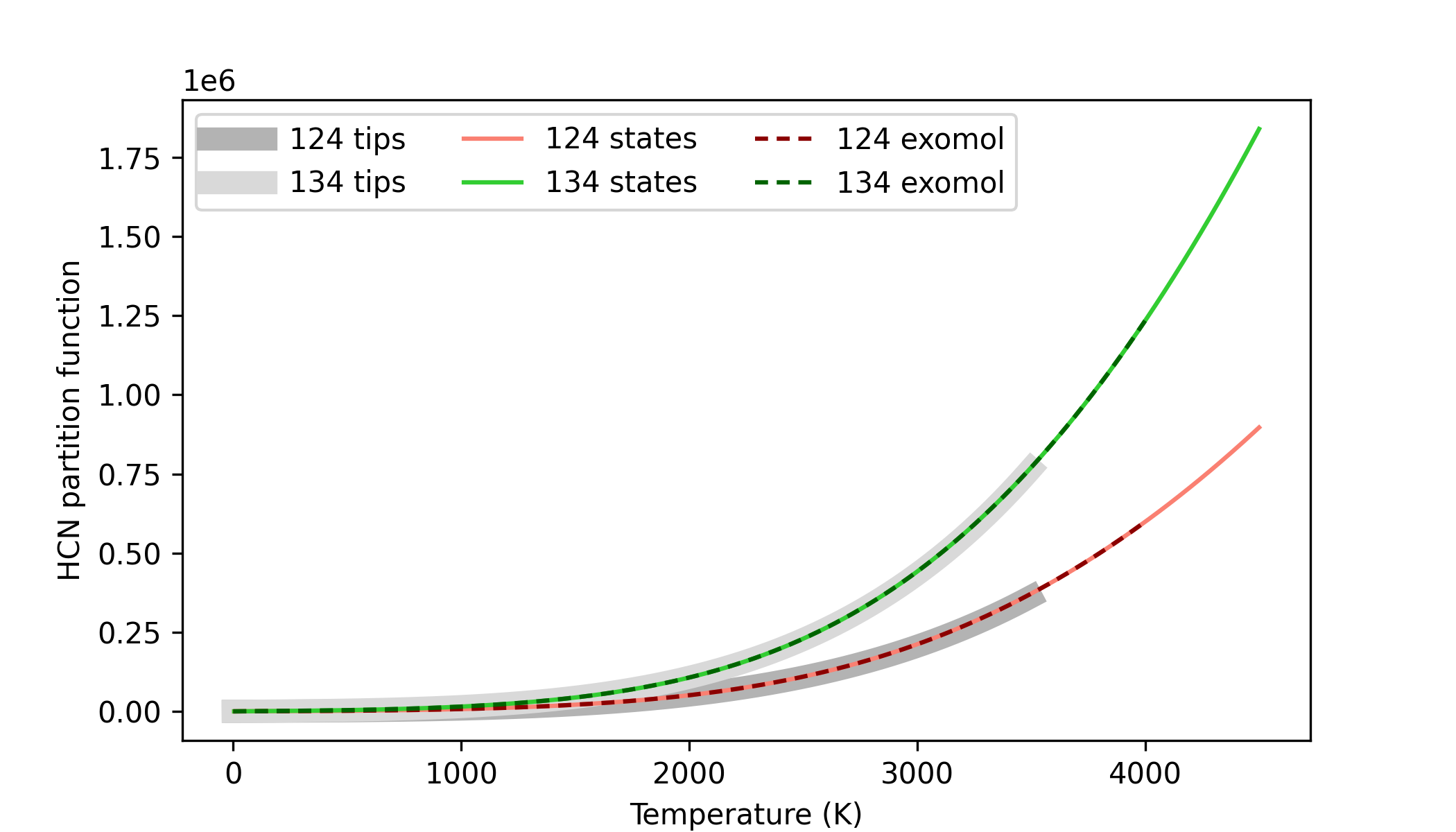
Here’s an interactive Python sctipt to compute partition functions for the HCN molecule:
import pyratbay.opacity.partitions as pf
import numpy as np
import matplotlib.pyplot as plt


# Compute HCN's partitions using all 3 available methods:
tips_pf, tips_iso, tips_temps = pf.tips('HCN')

exomol_pf = [
    '1H-12C-14N__Harris.pf',
    '1H-13C-14N__Larner.pf',
]
exomol_pf, exomol_iso, exomol_temps = pf.exomol_pf(exomol_pf)

exomol_states = [
    '1H-12C-14N__Harris.states',
    '1H-13C-14N__Larner.states',
]
states_pf, states_iso, states_temps = pf.exomol_states(
    exomol_states, tmin=5.0, tmax=4500.0, tstep=5.0,
)


# Plot and compare results
fig = plt.figure(0)
plt.clf()
fig.set_size_inches(7, 4)
plt.plot(tips_temps, tips_pf[0], lw=8, color='0.70', label='124 tips')
plt.plot(tips_temps, tips_pf[1], lw=8, color='0.85', label='134 tips')

plt.plot(states_temps, states_pf[0], color='salmon', label='124 states')
plt.plot(states_temps, states_pf[1], color='limegreen', label='134 states')

plt.plot(exomol_temps, exomol_pf[0], color='darkred', dashes=(3,2), label='124 exomol')
plt.plot(exomol_temps, exomol_pf[1], color='darkgreen', dashes=(3,2), label='134 exomol')
plt.legend(loc='upper left', ncol=3)
plt.xlabel('Temperature (K)')
plt.ylabel('HCN partition function')