Temperature profiles (basics)
This tutorial shows how to create and use temperature-pressure profiles. Currently, there are three temperature models:
Note
You can also find this tutorial as a jupyter notebook here.
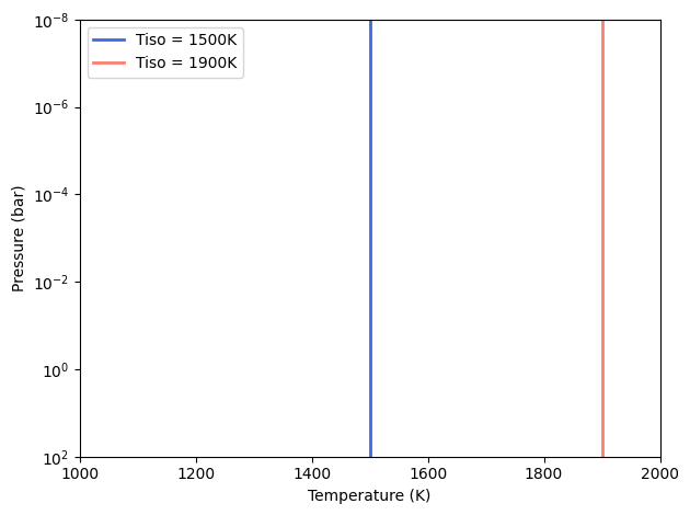
Isothermal Profiles
The isothermal model has a single free parameter (T_iso), which sets a constant temperature at all layers. Here is an example:
[1]:
import pyratbay.atmosphere as pa
import matplotlib.pyplot as plt
import numpy as np


# To initialize an isothermal model, provide the pressure array (bars):
pressure = pa.pressure(ptop='1e-8 bar', pbottom='100 bar', nlayers=61)
tp_iso = pa.tmodels.Isothermal(pressure)

# Evaluate a couple of TP profile at a given tempperature:
temp_iso_1500K = tp_iso(1500.0)
temp_iso_1900K = tp_iso(1900.0)


# Plot the results:
plt.figure(10)
plt.clf()
ax = plt.subplot(111)
ax.plot(temp_iso_1500K, pressure, color='royalblue', lw=2.0, label='Tiso = 1500K')
ax.plot(temp_iso_1900K, pressure, color='salmon', lw=2.0, label='Tiso = 1900K')
ax.set_yscale('log')
ax.set_ylim(np.amax(pressure), np.amin(pressure))
ax.set_xlabel('Temperature (K)')
ax.set_ylabel('Pressure (bar)')
ax.set_xlim(1000, 2000)
ax.legend()
plt.tight_layout()
[2]:
# This is some useful data contained in the object:
print(tp_iso)
Model name: isothermal
Number of parameters (npars): 1
Parameter names (pnames): ['T_iso']
Parameter Latex names (texnames): ['$T\\ ({\\rm K})$']
Pressure array (pressure, bar):
 [1.000e-08 1.468e-08 2.154e-08 3.162e-08 4.642e-08 6.813e-08 1.000e-07
 1.468e-07 2.154e-07 3.162e-07 4.642e-07 6.813e-07 1.000e-06 1.468e-06
 2.154e-06 3.162e-06 4.642e-06 6.813e-06 1.000e-05 1.468e-05 2.154e-05
 3.162e-05 4.642e-05 6.813e-05 1.000e-04 1.468e-04 2.154e-04 3.162e-04
 4.642e-04 6.813e-04 1.000e-03 1.468e-03 2.154e-03 3.162e-03 4.642e-03
 6.813e-03 1.000e-02 1.468e-02 2.154e-02 3.162e-02 4.642e-02 6.813e-02
 1.000e-01 1.468e-01 2.154e-01 3.162e-01 4.642e-01 6.813e-01 1.000e+00
 1.468e+00 2.154e+00 3.162e+00 4.642e+00 6.813e+00 1.000e+01 1.468e+01
 2.154e+01 3.162e+01 4.642e+01 6.813e+01 1.000e+02]
Last evaluated profile (temperature, K):
 [1900. 1900. 1900. 1900. 1900. 1900. 1900. 1900. 1900. 1900. 1900. 1900.
 1900. 1900. 1900. 1900. 1900. 1900. 1900. 1900. 1900. 1900. 1900. 1900.
 1900. 1900. 1900. 1900. 1900. 1900. 1900. 1900. 1900. 1900. 1900. 1900.
 1900. 1900. 1900. 1900. 1900. 1900. 1900. 1900. 1900. 1900. 1900. 1900.
 1900. 1900. 1900. 1900. 1900. 1900. 1900. 1900. 1900. 1900. 1900. 1900.
 1900.]
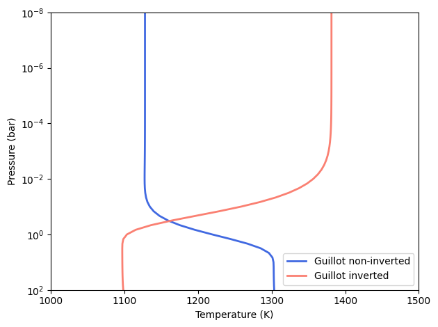
Guillot Profiles
The guillot model has six parameters as defined in Line et al. (2013):
log_kappa', log_gamma1, log_gamma2, alpha, T_irr, and T_int.
The temperature profile is defined as:
with
where \(E_{2}(\gamma_{i}\tau)\) is the second-order exponential integral; \(T_{\rm int}\) is the internal heat temperature; and \(\tau(p) = \kappa' p\) (note that this parameterization differs from that of Line et al. (2013), which are related as \(\kappa' \equiv \kappa/g\)). \(T_{\rm irr}\) parametrizes the stellar irradiation absorbed by the planet as:
Here’s a sample script:
[3]:
import pyratbay.atmosphere as pa
import matplotlib.pyplot as plt
import numpy as np


# To initialize a Guillot TP model, provide the pressure array (in bars):
pressure = pa.pressure(ptop='1e-8 bar', pbottom='100 bar', nlayers=61)
tp_guillot = pa.tmodels.Guillot(pressure)

# Evaluate a couple of Guillot profiles (non-inverted if log_gamma < 0):
# log_kappa', log_gamma1, log_gamma2, alpha, t_irr, t_int
params1 = -6.0, -0.25, 0.0, 0.0, 1200.0, 100.0
params2 = -6.0,  0.40, 0.0, 0.0, 1200.0, 100.0
temp_guillot1 = tp_guillot(params1)
temp_guillot2 = tp_guillot(params2)


# Plot the profiles:
plt.figure(20)
plt.clf()
ax = plt.subplot(111)
ax.plot(temp_guillot1, pressure, color='royalblue', lw=2.0, label='Guillot non-inverted')
ax.plot(temp_guillot2, pressure, color='salmon', lw=2.0, label='Guillot inverted')
ax.set_yscale('log')
ax.set_ylim(np.amax(pressure), np.amin(pressure))
ax.set_xlabel('Temperature (K)')
ax.set_ylabel('Pressure (bar)')
ax.set_xlim(1000, 1500)
ax.legend()
plt.tight_layout()
[4]:
# This is some useful data contained in the object:
print(tp_guillot)
Model name: guillot
Number of parameters (npars): 6
Parameter names (pnames): ["log_kappa'", 'log_gamma1', 'log_gamma2', 'alpha', 'T_irr', 'T_int']
Parameter Latex names (texnames): ["$\\log\\ \\kappa'$", '$\\log\\ \\gamma_1$', '$\\log\\ \\gamma_2$', '$\\alpha$', '$T_{\\rm irr} (K)$', '$T_{\\rm int} (K)$']
Pressure array (pressure, bar):
 [1.000e-08 1.468e-08 2.154e-08 3.162e-08 4.642e-08 6.813e-08 1.000e-07
 1.468e-07 2.154e-07 3.162e-07 4.642e-07 6.813e-07 1.000e-06 1.468e-06
 2.154e-06 3.162e-06 4.642e-06 6.813e-06 1.000e-05 1.468e-05 2.154e-05
 3.162e-05 4.642e-05 6.813e-05 1.000e-04 1.468e-04 2.154e-04 3.162e-04
 4.642e-04 6.813e-04 1.000e-03 1.468e-03 2.154e-03 3.162e-03 4.642e-03
 6.813e-03 1.000e-02 1.468e-02 2.154e-02 3.162e-02 4.642e-02 6.813e-02
 1.000e-01 1.468e-01 2.154e-01 3.162e-01 4.642e-01 6.813e-01 1.000e+00
 1.468e+00 2.154e+00 3.162e+00 4.642e+00 6.813e+00 1.000e+01 1.468e+01
 2.154e+01 3.162e+01 4.642e+01 6.813e+01 1.000e+02]
Last evaluated profile (temperature, K):
 [1381.37095226 1381.37090443 1381.37083585 1381.3707376  1381.3705969
 1381.37039556 1381.37010761 1381.3696961  1381.36910844 1381.36826986
 1381.36707422 1381.36537096 1381.36294678 1381.35949995 1381.35460413
 1381.34765794 1381.3378144  1381.32388272 1381.30419199 1381.27640248
 1381.23724531 1381.18216494 1381.10483001 1380.9964677  1380.84496273
 1380.63364577 1380.33967603 1379.93190036 1379.36804778 1378.59109637
 1377.52463564 1376.06705188 1374.08440422 1371.40196591 1367.79462787
 1362.97678349 1356.59307056 1348.21265984 1337.33199614 1323.39451071
 1305.84138649 1284.21503176 1258.34413805 1228.63574167 1196.45571889
 1164.43686627 1136.28854117 1115.56732886 1103.65360089 1098.75925501
 1097.48863344 1097.32337373 1097.33378615 1097.36441334 1097.40963114
 1097.47599247 1097.5733758  1097.71626804 1097.92590415 1098.23339057
 1098.68425169]
Further reading for the Guillot TP model:
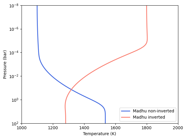
Madhu Profiles
The madhu model has six parameters as defined in Madhusudhan & Seager (2009):
log_p1, log_p2, log_p3, a1, a2, and T0
where the pressure values must be given in log10(bar) units. The temperature profile is then computed as a set to three layers given by:
A thermally inverted profile will result when \(p_1 < p_2\); a non-inverted profile will result when \(p_2 < p_1\).
Note
The pressure parameters must also satisfy: \(p_1 < p_3\) (otherwise the model will return zeros). In a retrieval you can use this as a condition to reject a proposed sample.
[5]:
import pyratbay.atmosphere as pa
import matplotlib.pyplot as plt
import numpy as np


# To initialize a Madhu model, provide the pressure array (in bars):
pressure = pa.pressure(ptop='1e-8 bar', pbottom='100 bar', nlayers=61)
tp_madhu = pa.tmodels.Madhu(pressure)


# Evaluate a couple of Madhu TP profiles (non-inverted if p1 > p2):
#      log_p1, log_p2, log_p3, a1, a2, T0
params1 = -3.5, -4.0, 0.5, 3.0, 0.5, 1100.0
params2 = -4.5, 0.5, 1.0, 3.0, 0.5, 1800.0
temp_madhu1 = tp_madhu(params1)
temp_madhu2 = tp_madhu(params2)


# Plot the profile:
plt.figure(30)
plt.clf()
ax = plt.subplot(111)
ax.plot(temp_madhu1, pressure, color='royalblue', lw=2.0, label='Madhu non-inverted')
ax.plot(temp_madhu2, pressure, color='salmon', lw=2.0, label='Madhu inverted')
ax.set_yscale('log')
ax.set_ylim(np.amax(pressure), np.amin(pressure))
ax.set_xlabel('Temperature (K)')
ax.set_ylabel('Pressure (bar)')
ax.set_xlim(1000, 2000)
ax.legend()
plt.tight_layout()
[6]:
# This is some useful data contained in the object:
print(tp_madhu)
Model name: madhu
Number of parameters (npars): 6
Parameter names (pnames): ['log_p1', 'log_p2', 'log_p3', 'a1', 'a2', 'T0']
Parameter Latex names (texnames): ['$\\log\\ p_1$', '$\\log\\ p_2$', '$\\log\\ p_3$', '$a_1$', '$a_2$', '$T_0$']
Pressure array (pressure, bar):
 [1.000e-08 1.468e-08 2.154e-08 3.162e-08 4.642e-08 6.813e-08 1.000e-07
 1.468e-07 2.154e-07 3.162e-07 4.642e-07 6.813e-07 1.000e-06 1.468e-06
 2.154e-06 3.162e-06 4.642e-06 6.813e-06 1.000e-05 1.468e-05 2.154e-05
 3.162e-05 4.642e-05 6.813e-05 1.000e-04 1.468e-04 2.154e-04 3.162e-04
 4.642e-04 6.813e-04 1.000e-03 1.468e-03 2.154e-03 3.162e-03 4.642e-03
 6.813e-03 1.000e-02 1.468e-02 2.154e-02 3.162e-02 4.642e-02 6.813e-02
 1.000e-01 1.468e-01 2.154e-01 3.162e-01 4.642e-01 6.813e-01 1.000e+00
 1.468e+00 2.154e+00 3.162e+00 4.642e+00 6.813e+00 1.000e+01 1.468e+01
 2.154e+01 3.162e+01 4.642e+01 6.813e+01 1.000e+02]
Last evaluated profile (temperature, K):
 [1800.0320672  1800.06719103 1800.12487823 1800.21001076 1800.32561448
 1800.4731641  1800.65322405 1800.86596372 1801.11142291 1801.38960892
 1801.7005227  1802.04416424 1802.42053355 1802.82963063 1803.26941797
 1803.72819719 1804.14777381 1804.30830458 1803.58545415 1800.67046615
 1793.61397366 1780.55500803 1760.84120201 1735.55888658 1706.91076749
 1677.05802248 1647.41263786 1618.63845855 1590.96718509 1564.45979785
 1539.12850688 1514.97541549 1492.00052368 1470.20383145 1449.58533879
 1430.14504572 1411.88295223 1394.79905832 1378.89336399 1364.16586924
 1350.61657407 1338.24547847 1327.05258246 1317.03788603 1308.20138918
 1300.54309191 1294.06299422 1288.76085917 1284.635251   1281.67889188
 1279.86353722 1279.1056873  1279.21881002 1279.892367   1280.75129945
 1281.48714928 1281.96201189 1282.19944506 1282.2921246  1282.32040324
 1282.32714227]
Further reading for the Madhu TP model: