Radiative equilibrium: WASP-69b
This tutorial shows how perform a radiative-equilibrium calculation to compute an exoplanet temperature profile. We will use WASP-69b as a test case.
Radiative-equilibrium estimations balance the incoming stellar irradiation from the host star and the outgoing planetary thermal emission. Thus, It’s important that the radiative-transfer calculation spans all the way from optical to infrared wavelengths, such that all relevant optical and infrared absorbers are included.
We can break the analysis into the following steps:
Cross sections
In this example we will include line-sampled cross sections for these molecules: H₂O, CO, CO₂, CH₄, SiO, H₂S, HCN, and NH₃. We will work with the latests opacity sources for these species from ExoMol, HITEMP, and Ames.
The Zenodo repository doi.org/10.5281/zenodo.16965391 provides the required cross-section files, ready to use. See the list below for direct links to the files for each molecule. These cross sections have been computed assuming an H₂/He-dominated atmosphere, and terrestrial isotopic ratios. The lines have Voigt profiles with a wing cut-off at 300 HWHM and at 25 cm-1. The grid sampling are:
Wavelength: \(0.15-33\) μm, at a constant resolution of \(R=25.000\)
Temperature: \(200-5000\) K, with \(\Delta T = 150\) K
Pressure: \(1.0^{-9}-1.0^{3}\) bar, equally sampled in log(p) with 4 samples per dex.
Species (source) |
References |
|---|---|
H2O (exomol, pokazatel) |
|
CO (HITEMP, li) |
|
CO2 (ames, ai3000k) |
|
CH4 (exomol, mm) |
|
H2S (exomol, ayt2) |
|
HCN (exomol, harris larner) |
|
NH3 (exomol, coyute) |
|
SiO (exomol, siouvenir) |
Note that these are mainly infrared abosrbers. Optical absorbers (e.g., Na, K, Rayleigh) will be defined later in the configuration file.
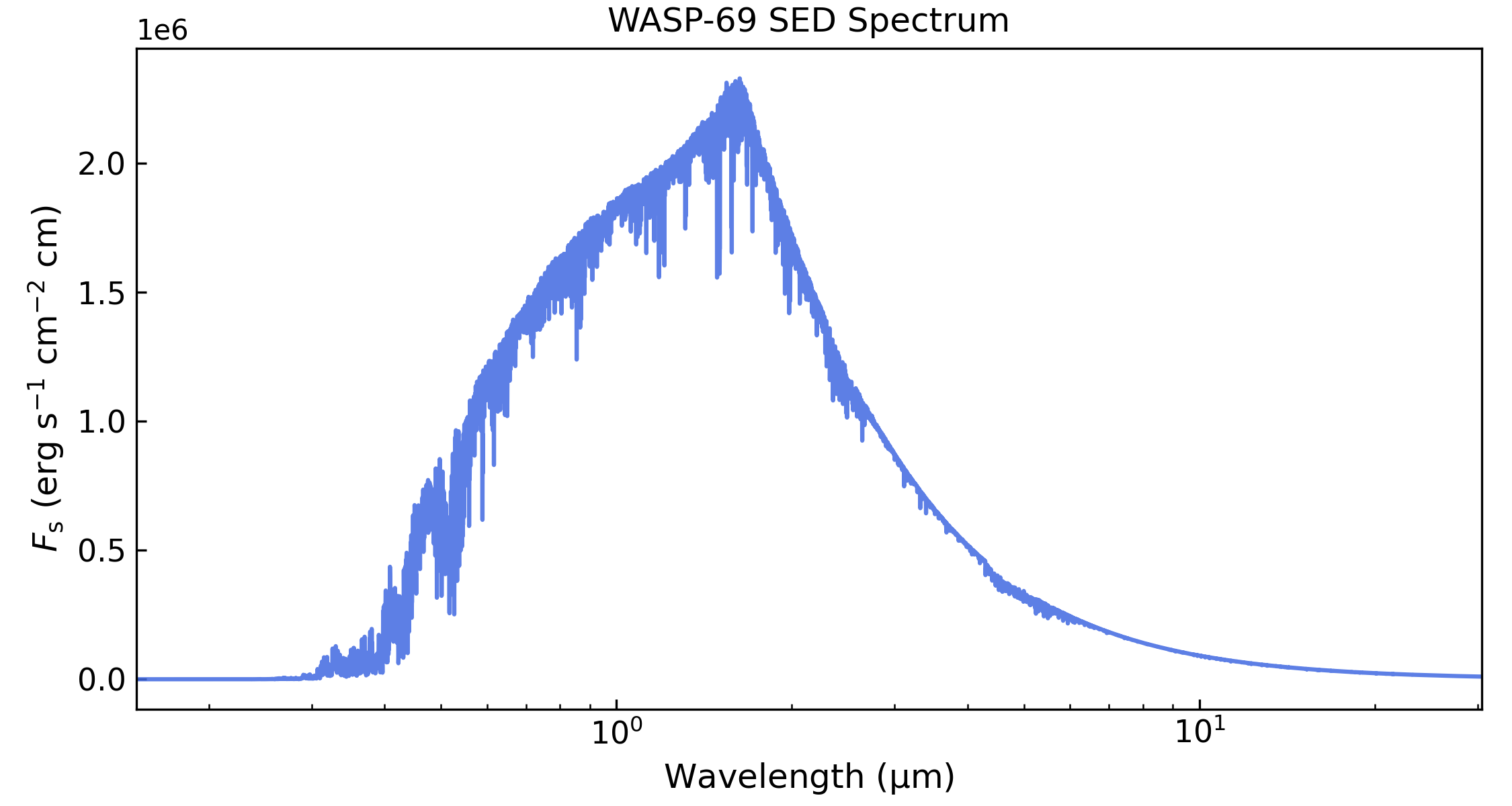
Stellar SED spectrum
The stellar spectral energy distribution (SED) sets the incident
irradiation at the top of the atmosphere, as a function of pressure.
Here we will make a stellar SED for WASP-69 from PHOENIX models
[Husser2013] using the Gen TSO package. If you haven’t already,
install this package with this shell command:
pip install gen_tso
Now, we can create the stellar SED spectrum with this Python script:
import gen_tso.pandeia_io as pandeia
import pyratbay.constants as pc
import pyratbay.spectrum as ps
import pyratbay.io as io
import matplotlib.pyplot as plt


# Use the Gen TSO package to get closest PHOENIX SED model for WASP-69
sed = pandeia.find_closest_sed(teff=4700, logg=4.5)
scene = pandeia.make_scene(
    sed_type='phoenix',
    sed_model=sed,
)
sed_wl, flux = pandeia.extract_sed(scene, wl_range=(0.15,35.0))

# Now convert flux from mJy to erg s-1 cm-2 cm
sed_flux = flux * pc.c / 1e26
# and lower the resolution
bin_wl = ps.constant_resolution_spectrum(0.15, 35.0, resolution=1500.0)
bin_sed_flux = ps.bin_spectrum(bin_wl, sed_wl, sed_flux, gaps='interpolate')

# Save to file
starspec_file = 'phoenix_WASP69b_4700K_logg4.5.dat'
io.write_spectrum(
    bin_wl,
    bin_sed_flux,
    starspec_file,
    type='emission',
)

# Lower the resolution to something more manageable
bin_wl = ps.constant_resolution_spectrum(0.15, 33.0, resolution=1500.0)
bin_sed_flux = ps.bin_spectrum(bin_wl, sed_wl, sed_flux, gaps='interpolate')

# Take a look
plt.figure(0, (7.5, 4.0))
plt.clf()
plt.subplots_adjust(0.09, 0.12, 0.98, 0.94)
ax = plt.subplot(111)
ax.plot(bin_wl, bin_sed_flux, color='royalblue', alpha=0.85)
ax.set_title('WASP-69 SED Spectrum')
ax.set_xscale('log')
ax.set_xlim(0.15, 30.5)
ax.set_xlabel(r'Wavelength ($\mathrm{\mu}$m)', fontsize=12)
ax.set_ylabel(r'$F_{\rm s}$ (erg s$^{-1}$ cm$^{-2}$ cm)', fontsize=12)
ax.tick_params(direction='in', which='both', labelsize=11)
Configuration file
Lastly, the configuration file will put together the inputs, define system and atmospheric properties, and set the radiative-equilibrium configuration. Here is the file we will use for the WASP-69b simulation.
Click here to show/hide: wasp69b_radeq_1x_solar_metallicity.cfg
[pyrat]

# Pyrat Bay run mode [tli atmosphere opacity spectrum radeq retrieval]
runmode = radeq
# Number of radiative-equilibrium iterations
nsamples = 250

# Output file names
logfile = radeq_WASP69b_1x_solar_metallicity.log

# Verbosity level [1--3]
verb = 2

# Observing geometry, select between: [transit eclipse emission_two_stream]
rt_path = emission_two_stream

# Wavelength sampling
wl_low = 0.15 um
wl_high = 33.0 um
wl_thinning = 2

# System parameters (Bonomo et al. 2017)
rstar = 0.813 rsun
mstar = 0.826 msun
starspec = inputs/phoenix_WASP69b_4700K_logg4.5.dat

rplanet = 1.057 rjup
mplanet = 0.250 mjup
smaxis = 0.04527 au
refpressure = 1e-2 bar

# Atmospheric model
ptop = 1.0e-9 bar
pbottom = 100 bar
nlayers = 81

# Initial thermal profile for radiative-equilibrium runs
tmodel = isothermal
tpars = 900.0

# Chemistry and composition
chemistry = equilibrium
species =
    H  He  C  N  O  Na  K  Mg  Si  P  S  Cl Ti  V Fe
    H2  H2O  CH4  CO  CO2  HCN  NH3  N2  OH  C2H2  C2H4
    S2  SH  H2S  SO2  SO  TiO  VO  TiO2  VO2   SiO  SiH  SiS  SiH4
    OCS PH PH3 PN PO KOH CS CS2 NaH  NaCl  HCl  KCl NaOH
    e-  H-  H+  H2+  He+  Na-  Na+  Mg+ K-  K+  Fe+  Ti+  V+  SiH+ Si- Si+
# Elemental composition
vmr_vars =
    [M/H] 0.0
    C/O 0.59

# Hydrostatic equilibrium
radmodel = hydro_m

# Stellar irradiation scaling factor, beta = (1-A)*f
beta_irr = 0.66

# Internal heat (K)
tint = 100.0

# Line-by-line sampled cross sections
sampled_cross_sec =
    inputs/cross_section_0.15-33.0um_0200-5000K_R025K_H2O_exomol_pokazatel.npz
    inputs/cross_section_0.15-33.0um_0200-5000K_R025K_CO_hitemp_2019.npz
    inputs/cross_section_0.15-33.0um_0200-5000K_R025K_CO2_ames_ai3000k.npz
    inputs/cross_section_0.15-33.0um_0200-5000K_R025K_CH4_exomol_mm.npz
    inputs/cross_section_0.15-33.0um_0200-5000K_R025K_H2S_exomol_ayt2.npz
    inputs/cross_section_0.15-33.0um_0200-5000K_R025K_HCN_exomol_harris_larner.npz
    inputs/cross_section_0.15-33.0um_0200-5000K_R025K_NH3_exomol_coyute.npz
    inputs/cross_section_0.15-33.0um_0200-5000K_R025K_SiO_exomol_siouvenir.npz

# Alkali models, select from: [sodium_vdw potassium_vdw]
alkali =
    sodium_vdw
    potassium_vdw

# Continuum cross sections
continuum_cross_sec =
    {ROOT}/pyratbay/data/CIA/CIA_Borysow_H2H2_0060-7000K_0.6-500um.dat
    {ROOT}/pyratbay/data/CIA/CIA_Borysow_H2He_0050-7000K_0.5-031um.dat

# Rayleigh models, select from: [rayleigh_H rayleigh_He rayleigh_H2]
rayleigh =
    rayleigh_H2
    rayleigh_He
    rayleigh_H

# H- continous absorption
h_ion = h_ion_john1988
Lets break this down:
# Pyrat Bay run mode [tli atmosphere opacity spectrum radeq retrieval]
runmode = radeq
# Number of radiative-equilibrium iterations
nsamples = 250

# Output file names
logfile = radeq_WASP69b_1x_solar_metallicity.log

# Verbosity level [1--3]
verb = 2
This first section defines what we want to run. runmode =
radeq indicates that we want a radiative-equilibrium
calculation. nsamples set the number of
radiative-equilibrium iterations to run. logfile sets the
path to the output files (logs, temperature profile, and emission
spectrum). Finally, verb sets the screen-output verbosity.
# Observing geometry, select between: [transit eclipse emission_two_stream]
rt_path = emission_two_stream

# Wavelength sampling
wl_low = 0.15 um
wl_high = 33.0 um
wl_thinning = 2
Here we define the observing path and radiative-transfer scheme.
For radiative-equilibrium runs set rt_path =
emission_two_stream to compute the upward/downward emission
through the atmosphere.
The wavelength sampling rate and coverage is set by the
sampled_cross_section files. The wl_low and wl_high
variables help to trim down the wavelength range (though in this
case we keep the wavelength range as wide as possible). Setting
a wl_thinning = n parameter lowers the resolution by taking
every n-th spectral sample (with n an integer). Here we
reduce the sampling resolution by a factor of two to speed up the
runs.
# System parameters (Bonomo et al. 2017)
rstar = 0.813 rsun
mstar = 0.826 msun
starspec = inputs/phoenix_WASP69b_4700K_logg4.5.dat

rplanet = 1.057 rjup
mplanet = 0.250 mjup
smaxis = 0.04527 au
refpressure = 1e-2 bar
And this next section defines the system parameters. For a radiative-equilibrium run, the most relevant properties will be the stellar radius, the orbital semi-major axis, and the stellar SED. These parameters set the incident irradiation at the top of the atmosphere.
The other relevant planetary parameters set the planet mass, the
planet radius, and the pressure at the given planet radius
(refpressure).
# Atmospheric model
ptop = 1.0e-9 bar
pbottom = 100 bar
nlayers = 81

# Initial thermal profile for radiative-equilibrium runs
tmodel = isothermal
tpars = 900.0

# Chemistry and composition
chemistry = equilibrium
species =
    H  He  C  N  O  Na  K  Mg  Si  P  S  Cl Ti  V Fe
    H2  H2O  CH4  CO  CO2  HCN  NH3  N2  OH  C2H2  C2H4
    S2  SH  H2S  SO2  SO  TiO  VO  TiO2  VO2   SiO  SiH  SiS  SiH4
    OCS PH PH3 PN PO KOH CS CS2 NaH  NaCl  HCl  KCl NaOH
    e-  H-  H+  H2+  He+  Na-  Na+  Mg+ K-  K+  Fe+  Ti+  V+  SiH+ Si- Si+
# Elemental composition
vmr_vars =
    [M/H] 0.0
    C/O 0.59

# Hydrostatic equilibrium
radmodel = hydro_m
These parameters define the atmospheric profile models. For the
pressure range, the only constraint is that the bottom boundary
(i.e., max pressure) must be covered by the
sampled_cross_section files.
Note that the temperature profile parameters define the starting point for the radiative-equilibrium calculation. The recommendation is to start with an isothermal profile at the equilibrium temperature.
For the composition, thermochemical equilibrium is the
recommendation. Here it’s important to include all species that
can be chemically relevant across the range of temperatures and
pressures. vmr_vars allows one to customize elemental
composition and ratios that differ from the solar values if
needed.
radmodel tells the code to compute the atmospheric layers’
altitude under hydrostatic equilibrium assuming \(g(r) =
GM/r^2\) and boundary condition from rplanet and
refpressure (\(r(p_{\rm ref}) = r_{\rm p}\)).
# Stellar irradiation scaling factor, beta = (1-A)*f
beta_irr = 0.66

# Internal heat (K)
tint = 100.0
Finally, these pair of variables define the radiative boundary
conditions at the top of the atmosphere. tint is the
internal heat from the planet at the bottom of the
atmosphere. beta_irr sets how much stellar irradiation is
absorbed at the top of the atmosphere:
where \(a\) is the semi-major axis, \(R_*\) the stellar radius, and \(F_*\) the stellar SED.
# Line-by-line sampled cross sections
sampled_cross_sec =
    inputs/cross_section_0.15-33.0um_0200-5000K_R025K_H2O_exomol_pokazatel.npz
    inputs/cross_section_0.15-33.0um_0200-5000K_R025K_CO_hitemp_2019.npz
    inputs/cross_section_0.15-33.0um_0200-5000K_R025K_CO2_ames_ai3000k.npz
    inputs/cross_section_0.15-33.0um_0200-5000K_R025K_CH4_exomol_mm.npz
    inputs/cross_section_0.15-33.0um_0200-5000K_R025K_H2S_exomol_ayt2.npz
    inputs/cross_section_0.15-33.0um_0200-5000K_R025K_HCN_exomol_harris_larner.npz
    inputs/cross_section_0.15-33.0um_0200-5000K_R025K_NH3_exomol_coyute.npz
    inputs/cross_section_0.15-33.0um_0200-5000K_R025K_SiO_exomol_siouvenir.npz

# Alkali models, select from: [sodium_vdw potassium_vdw]
alkali =
    sodium_vdw
    potassium_vdw

# Continuum cross sections
continuum_cross_sec =
    {ROOT}/pyratbay/data/CIA/CIA_Borysow_H2H2_0060-7000K_0.6-500um.dat
    {ROOT}/pyratbay/data/CIA/CIA_Borysow_H2He_0050-7000K_0.5-031um.dat

# Rayleigh models, select from: [rayleigh_H rayleigh_He rayleigh_H2]
rayleigh =
    rayleigh_H2
    rayleigh_He
    rayleigh_H

# H- continous absorption
h_ion = h_ion_john1988
This section defines the atmospheric absorbers. Make sure that
all absorber species are defined in the atmospheric composition.
Note that some of these set constraints to the domain to be
explored. The sampled_cross_sec files set the maximum
resolution, spectral range, temperature range, and pressure. The
continuum_cross_sec files set temperature range constraints,
but one can span beyond their wavelength ranges.
On top of the line-sampled opacities, we add Na and K alkali models from [Burrows2000]; H₂-H₂ and H₂-He CIA; and H, H₂, and He Rayleigh opacities.
Radiative-equilibrium run
To launch the radiative-equilibrium run, use the following prompt command:
# Run radiative-equilibrium calculation
pbay -c wasp69b_radeq_1x_solar_metallicity.cfg
That’s it. This should take a couple of minutes to complete the iterations. The progress will be displayed on screen. Once finished, this run will produce four files:
radeq_WASP69b_1x_solar_metallicity.atm: Atmospheric profile at last iteration (p, T, VMRs)radeq_WASP69b_1x_solar_metallicity.dat: Planetary emission spectrum at final iterationradeq_WASP69b_1x_solar_metallicity.npz: Temperature profile at each iterationradeq_WASP69b_1x_solar_metallicity.log: Screen-output log
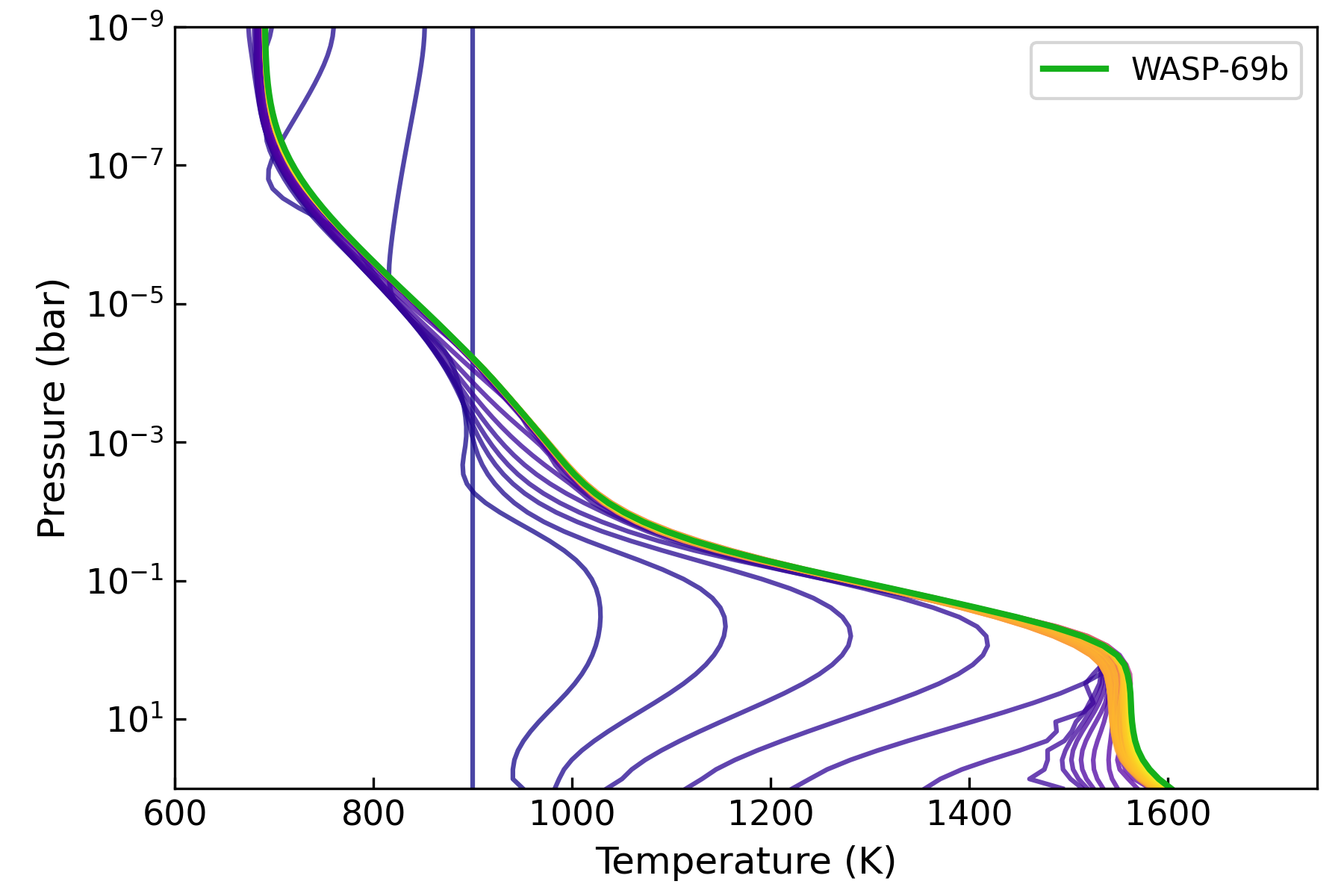
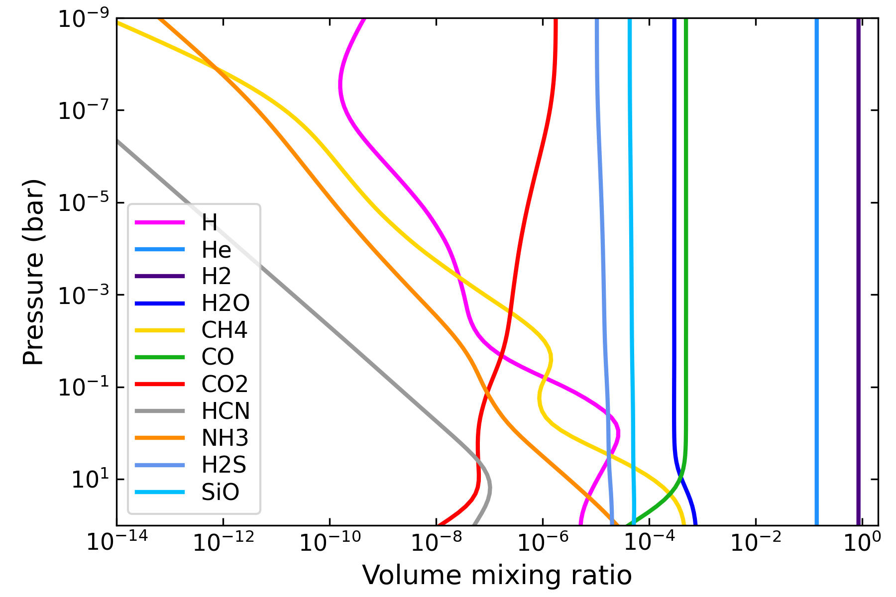
Radiative equilibrium profiles will typically settle after a couple hundred iterations. These Python scripts show how the temperature converges toward radiative equilibrium (purple to yellow to green profiles), and the resulting abundances corresponding to the final iteration:
import pyratbay.io as io
import pyratbay.plots as pp
import numpy as np
import matplotlib.pyplot as plt
plt.ion()

# Temperature profiles
file = 'radeq_WASP69b_1x_solar_metallicity.npz'
data = np.load(file)
press = data['pressure']
temps = data['temps']
niter, nlay = np.shape(temps)

# Abundances
a_file = 'radeq_WASP69b_1x_solar_metallicity.atm'
units, species, press, temp, vmr, rad = io.read_atm(a_file)

fig = plt.figure(1)
plt.clf()
fig.set_size_inches(5.25, 4)
ax = plt.subplots_adjust(0.13, 0.12, 0.98, 0.97)
ax = plt.subplot(111)
for i in range(0, niter, 3):
    c = i / niter
    ax.plot(temps[i], press, c=plt.cm.plasma(c), alpha=0.75)
ax.plot(temps[niter-1], press, label='WASP-69b', c='xkcd:green', lw=2)
ax.set_xlabel('Temperature (K)', fontsize=12)
ax.set_ylabel('Pressure (bar)', fontsize=12)
ax.legend(loc='upper right')
ax.tick_params(direction='in', which='both', labelsize=11)
ax.set_yscale('log')
ax.set_ylim(100, 1e-9)
ax.set_xlim(600, 1750)

# Only show molecules of interest
mol_show = ['H2', 'He', 'H', 'H2O', 'CO', 'CO2', 'CH4', 'H2S', 'HCN', 'NH3', 'SiO']
imol = np.isin(species, mol_show)
fig = plt.figure(2)
plt.clf()
fig.set_size_inches(6, 4)
ax = plt.subplot(111)
plt.subplots_adjust(0.13, 0.12, 0.98, 0.97)
ax = pp.abundance(
    vmr[:,imol], press, species[imol],
    colors='default', xlim=[1e-14, 2.0], ax=ax,
)
|
|
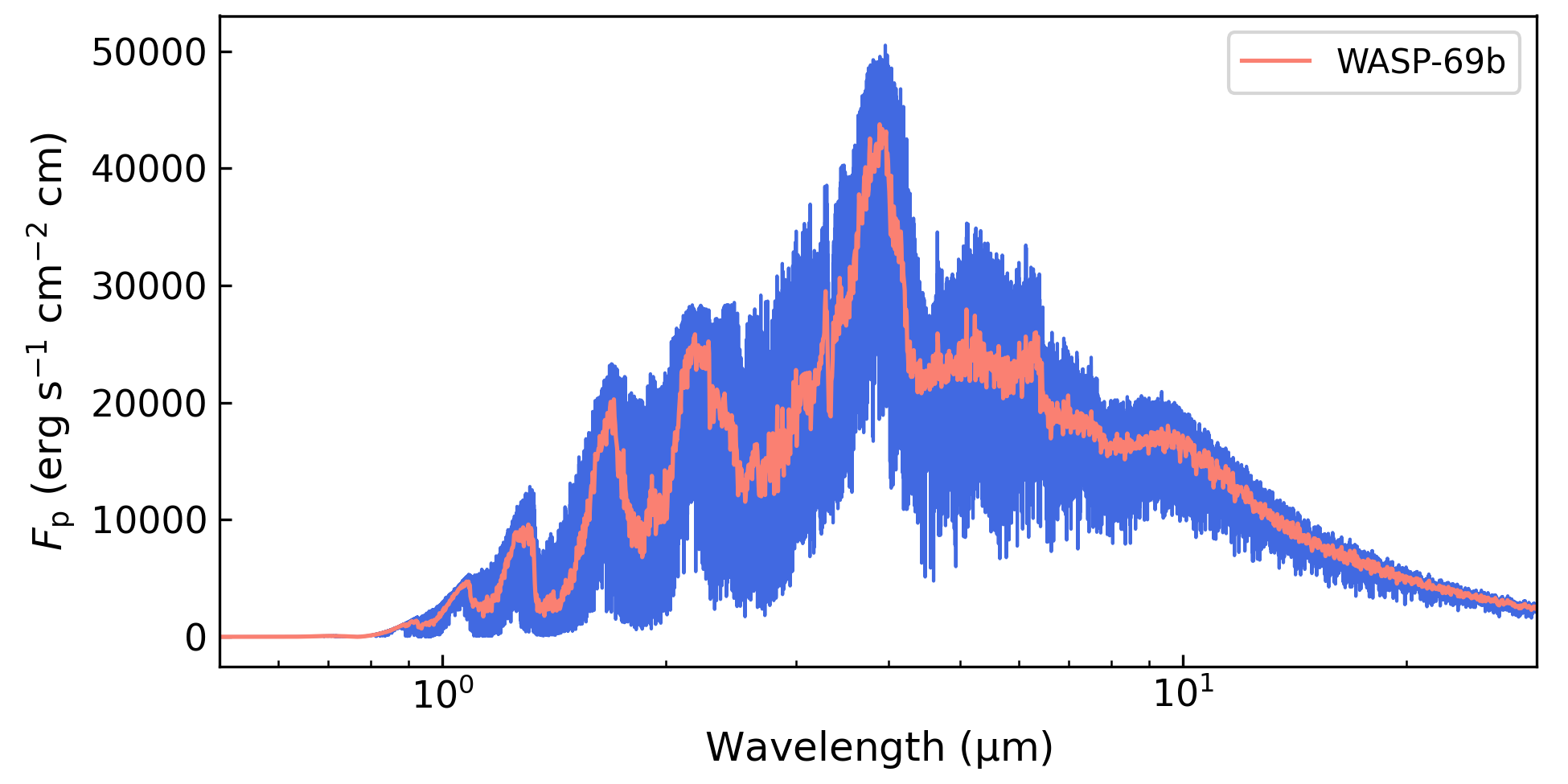
And we also have the planetary emission spectrum from the top of the atmosphere:
import numpy as np
import pyratbay.spectrum as ps
import matplotlib.pyplot as plt
plt.ion()

s_file = 'radeq_WASP69b_1x_solar_metallicity.dat'
wl, p_flux = np.loadtxt(s_file, unpack=True)
bin_wl = ps.constant_resolution_spectrum(0.5, 30.0, resolution=500.0)
bin_pflux = ps.bin_spectrum(bin_wl, wl, p_flux)

fig = plt.figure(3)
plt.clf()
fig.set_size_inches(6.5, 3.25)
ax = plt.subplots_adjust(0.14, 0.15, 0.98, 0.98)
ax = plt.subplot(111)
ax.plot(wl, p_flux, label='WASP-69b', c='royalblue', lw=1.0)
ax.plot(bin_wl, bin_pflux, c='salmon', lw=1.25)
ax.legend(loc='upper right')
ax.set_xscale('log')
ax.set_xlim(0.5, 30.0)
ax.set_xlabel(r'Wavelength ($\mathrm{\mu}$m)', fontsize=12)
ax.set_ylabel(r'$F_{\rm p}$ (erg s$^{-1}$ cm$^{-2}$ cm)', fontsize=12)
ax.tick_params(direction='in', which='both', labelsize=11)