Rayleigh opacities tutorial

This tutorial shows how to create Rayleigh opacity objects and compute their extinction coefficient spectra for a given atmospheric profile.

Note

You can also find this tutorial as a jupyter notebook here.

# Lets start by importing some useful modules
import pyratbay.atmosphere as pa
import pyratbay.spectrum as ps
import pyratbay.opacity as op

import matplotlib.pyplot as plt
import matplotlib
import numpy as np

H, H2, and He models

# We will sample the opacity over a constant-resolution wavelength array
# (boundaries in micron units)
wl_min = 0.2
wl_max = 6.0
resolution = 15000.0
wl = ps.constant_resolution_spectrum(wl_min, wl_max, resolution)

# Models for H, H2, and He based on Dalgarno models (from Kurucz 1970)
H2_rayleigh = op.rayleigh.Kurucz(wn=1e4/wl, species='H2')

# A print() call shows some useful info about the object:
print(H2_rayleigh)

Model name (name): 'rayleigh_H2'
Model species (species): H2
Number of model parameters (npars): 0
Wavenumber (wn, cm-1):
   [50000.00 49996.67 49993.33 ... 1667.00 1666.88 1666.77]
Cross section (cross_section, cm2 molec-1):
   [7.716e-26 7.714e-26 7.711e-26 ... 6.289e-32 6.287e-32 6.285e-32]

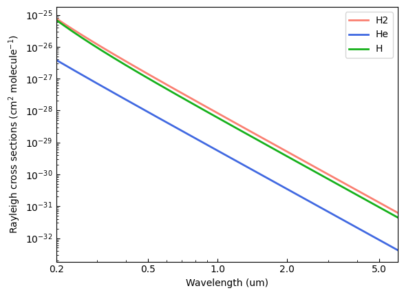
# Show the Rayleigh cross-section spectra
He_rayleigh = op.rayleigh.Kurucz(wn=1e4/wl, species='He')
H_rayleigh = op.rayleigh.Kurucz(wn=1e4/wl, species='H')

plt.figure(2)
plt.clf()
ax = plt.subplot(111)
ax.plot(wl, H2_rayleigh.cross_section, color='salmon', lw=2.0, label='H2')
ax.plot(wl, He_rayleigh.cross_section, color='royalblue', lw=2.0, label='He')
ax.plot(wl, H_rayleigh.cross_section, color='xkcd:green', lw=2.0, label='H')
ax.set_xscale('log')
ax.set_yscale('log')
ax.set_xlim(np.amin(wl), np.amax(wl))
ax.set_xlabel('Wavelength (um)')
ax.xaxis.set_major_formatter(matplotlib.ticker.ScalarFormatter())
ax.set_xticks([0.2, 0.5, 1.0, 2.0, 5.0])
ax.tick_params(which='both', direction='in')
ax.set_ylabel('Rayleigh cross sections (cm$^{2}$ molecule$^{-1}$)')
ax.legend(loc='upper right')

<matplotlib.legend.Legend at 0x79e60de876e0>

# Now a more practical example, compute the extinction coefficient
# across an atmosphere:

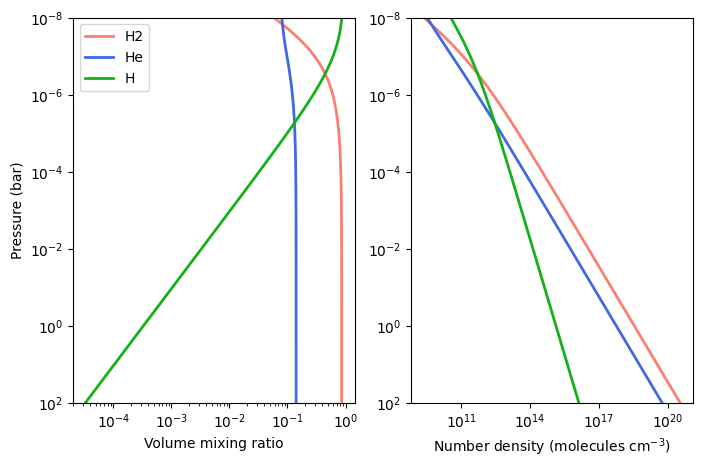
# First, let's consider a simple solar-abundance isothermal atmosphere
nlayers = 81
pressure = pa.pressure('1e-8 bar', '1e2 bar', nlayers)
temperature = np.tile(1800.0, nlayers)

# And a simple thermochemical equilibrium composition (only H2, H, and He)
species = ['H2', 'He', 'H']
net, species, vmr = pa.chemistry('equilibrium', pressure, temperature, species)
# Number-density profiles under IGL (molecules per cm3)
number_densities = pa.ideal_gas_density(vmr, pressure, temperature)

H2_number_density = number_densities[:,0]
He_number_density = number_densities[:,1]
H_number_density = number_densities[:,2]


# Show profiles:
cols = ['salmon', 'royalblue', 'xkcd:green']
plt.figure(1, (8,5))
plt.clf()
ax = plt.subplot(121)
for i, spec in enumerate(species):
    ax.plot(vmr[:,i], pressure, color=cols[i], lw=2.0, label=spec)
ax.set_xscale('log')
ax.set_yscale('log')
ax.set_ylim(100, 1e-8)
ax.set_xlabel('Volume mixing ratio')
ax.set_ylabel('Pressure (bar)')
ax.legend(loc='best')

ax = plt.subplot(122)
for i, spec in enumerate(species):
    ax.plot(number_densities[:,i], pressure, color=cols[i], lw=2.0, label=spec)
ax.set_xscale('log')
ax.set_yscale('log')
ax.set_ylim(100, 1e-8)
ax.set_xlabel('Number density (molecules cm$^{-3}$)')

Compute chemical abundances.

Text(0.5, 0, 'Number density (molecules cm$^{-3}$)')

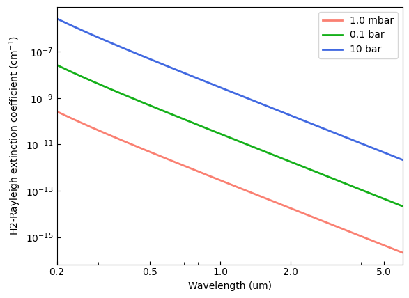
# Calculate extinction-coefficient spectra (cm-1) over the profile
H2_ec = H2_rayleigh.calc_extinction_coefficient(H2_number_density)

plt.figure(2)
plt.clf()
ax = plt.subplot(111)
ax.plot(wl, H2_ec[40], color='salmon', lw=2.0, label='1.0 mbar')
ax.plot(wl, H2_ec[56], color='xkcd:green', lw=2.0, label='0.1 bar')
ax.plot(wl, H2_ec[72], color='royalblue', lw=2.0, label='10 bar')
ax.set_xscale('log')
ax.set_yscale('log')
ax.set_xlim(np.amin(wl), np.amax(wl))
ax.set_xlabel('Wavelength (um)')
ax.xaxis.set_major_formatter(matplotlib.ticker.ScalarFormatter())
ax.set_xticks([0.2, 0.5, 1.0, 2.0, 5.0])
ax.tick_params(which='both', direction='in')
ax.set_ylabel('H2-Rayleigh extinction coefficient (cm$^{-1}$)')
ax.legend(loc='upper right')

<matplotlib.legend.Legend at 0x79e60d66caa0>