Line-sample Opacity Tutorial

This tutorial shows how to create a line-sample opacity object and compute extinction coefficient spectra for a given atmospheric profile.

As inputs for this demo we will use the tabulated cross sections for H2O and CO from HITRAN/HITEMP. To generate these inputs, run the script in Sample HITRAN/HITEMP line lists so that you have the following files in your current directory:

• cross_section_R020K_0150-3000K_0.5-5.0um_hitran_H2O.npz

• cross_section_R020K_0150-3000K_0.5-5.0um_hitemp_CO.npz

Note

You can also find this tutorial as a Python script here or as a jupyter notebook here.

# Lets start by importing some necessary modules
import pyratbay.opacity as op
import pyratbay.atmosphere as pa
import pyratbay.constants as pc

import numpy as np
import matplotlib.pyplot as plt


# Load up HITRAN H2O and CO line-sampling opacities:
cs_files = [
    'cross_section_R020K_0150-3000K_0.5-5.0um_hitran_H2O.npz',
    'cross_section_R020K_0150-3000K_0.5-5.0um_hitemp_CO.npz',
]

# Initialize line-sample object:
line_sample = op.Line_Sample(cs_files)

# A print() call shows some useful info about the object:
print(line_sample)

Line-sampling cross-section files (cs_files):
['cross_section_R020K_0150-3000K_0.5-5.0um_hitran_H2O.npz',
    'cross_section_R020K_0150-3000K_0.5-5.0um_hitemp_CO.npz']
Number of species (nspec): 2
Number of temperature samples (ntemp): 20
Number of pressure layers (nlayers): 51
Number of wavenumber samples (nwave): 46052

Minimum and maximum temperatures (tmin, tmax) in K: [150.0, 3000.0]
Minimum and maximum pressures in bar: [1.000e-08, 1.000e+02]
Minimum and maximum wavelengths in um: [0.500, 5.000]

Line-sample species (species): ['H2O' 'CO']
Temperature array (temps, K):
[ 150.  300.  450.  600.  750.  900. 1050. 1200. 1350. 1500. 1650. 1800.
 1950. 2100. 2250. 2400. 2550. 2700. 2850. 3000.]
Pressure layers (pressure, bar):
[1.000e-08 1.585e-08 2.512e-08 3.981e-08 6.310e-08 1.000e-07 1.585e-07
 2.512e-07 3.981e-07 6.310e-07 1.000e-06 1.585e-06 2.512e-06 3.981e-06
 6.310e-06 1.000e-05 1.585e-05 2.512e-05 3.981e-05 6.310e-05 1.000e-04
 1.585e-04 2.512e-04 3.981e-04 6.310e-04 1.000e-03 1.585e-03 2.512e-03
 3.981e-03 6.310e-03 1.000e-02 1.585e-02 2.512e-02 3.981e-02 6.310e-02
 1.000e-01 1.585e-01 2.512e-01 3.981e-01 6.310e-01 1.000e+00 1.585e+00
 2.512e+00 3.981e+00 6.310e+00 1.000e+01 1.585e+01 2.512e+01 3.981e+01
 6.310e+01 1.000e+02]
Wavenumber array (wn, cm-1):
  [ 2000.     2000.1    2000.2   ... 19997.298 19998.298 19999.298]
The tabulated cross sections (cs_table, cm2 molecule-1) are an array
of dimensions [nspec,ntemp,nlayers,nwave] and shape (2, 20, 51, 46052)

Compute spectra

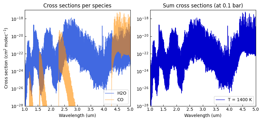
Lets compute some cross-section and extinction coefficients for an atmosphere model:

# Calculate cross sections:
temperature = np.tile(1400.0, line_sample.nlayers)
cross_section = line_sample.calc_cross_section(temperature)

# Set the flag per_mol=True to request cross sections per molecule:
cs_per_mol = line_sample.calc_cross_section(temperature, per_mol=True)


# Show cross sections at this layer (0.1 bar):
i_press = 35
pressure = line_sample.press
wl = line_sample.get_wl('um')

plt.figure(1, (8.5, 4.0))
plt.clf()
ax = plt.subplot(121)
ax.plot(wl, cs_per_mol[0,i_press], color='royalblue', lw=1.0, label='H2O')
ax.plot(wl, cs_per_mol[1,i_press], color='darkorange', lw=1.0, label='CO', alpha=0.6)
ax.set_yscale('log')
ax.set_ylabel('Cross section (cm$^{2}$ molec$^{-1}$)')
ax.set_xlabel('Wavelength (um)')
ax.set_xlim(1.0, 5.0)
ax.set_ylim(1e-28, 1e-17)
ax.tick_params(which='both', direction='in')
ax.set_title('Cross sections per species')
ax.legend(loc='lower right')

ax = plt.subplot(122)
ax.plot(wl, cross_section[i_press], color='mediumblue', lw=1.0, label='T = 1400 K')
ax.set_yscale('log')
ax.set_xlabel('Wavelength (um)')
ax.set_xlim(1.0, 5.0)
ax.set_ylim(1e-28, 1e-17)
ax.tick_params(which='both', direction='in')
ax.set_title(f'Sum cross sections (at {pressure[i_press]} bar)')
ax.legend(loc='lower right')
plt.tight_layout()

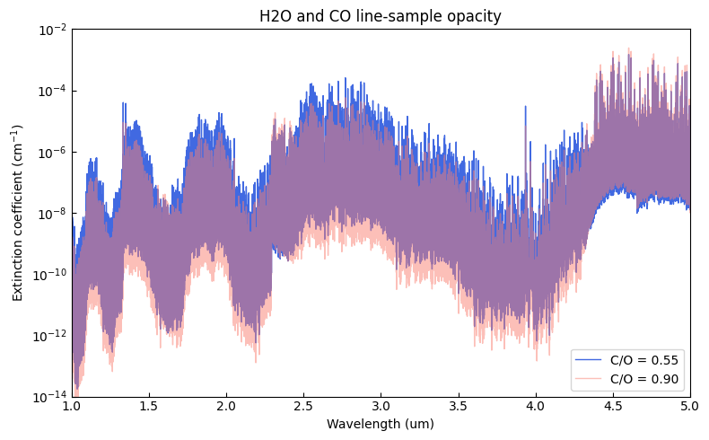
# Likewise, we can calculate extinction coefficients by providing a
# temperature and number density profile:

# Consider a simplified solar-abundance isothermal atmosphere
pressure = line_sample.press
temperature = np.tile(1400.0, line_sample.nlayers)
species = ['H2', 'H', 'He', 'H2O', 'CO', 'CO2', 'CH4']
chemistry = pa.chemistry('tea', pressure, temperature, species)

# Equilibrium abundances for solar and super-solar C/O ratios:
vmr_solar = chemistry.thermochemical_equilibrium(e_ratio={'C_O': 0.55})
vmr_super = chemistry.thermochemical_equilibrium(e_ratio={'C_O': 0.9})

# Number-density profiles under IGL (molecules per cm3)
densities_solar = pa.ideal_gas_density(vmr_solar, pressure, temperature)
densities_super = pa.ideal_gas_density(vmr_super, pressure, temperature)

# Indices for line-sample species in the atmosphere:
i_mol = [species.index(mol) for mol in line_sample.species]


# Compute extinction:
extinction_solar = line_sample.calc_extinction_coefficient(
    temperature, densities_solar[:,i_mol],
)
extinction_super = line_sample.calc_extinction_coefficient(
    temperature, densities_super[:,i_mol],
)

plt.figure(2, (8,5))
plt.clf()
ax = plt.subplot(111)
ax.plot(wl, extinction_solar[i_press], color='royalblue', lw=1.0, label='C/O = 0.55')
ax.plot(wl, extinction_super[i_press], color='salmon', lw=1.0, label='C/O = 0.90', alpha=0.5)
ax.set_yscale('log')
ax.set_xlabel('Wavelength (um)')
ax.set_xlim(1.0, 5.0)
ax.set_ylim(1.0e-14, 1e-2)
ax.tick_params(which='both', direction='in')
ax.set_ylabel('Extinction coefficient (cm$^{-1}$)')
ax.legend(loc='lower right')
ax.set_title('H2O and CO line-sample opacity')
plt.tight_layout()

Compute chemical abundances.

Customize cross-section grid

On initialization the user can set the wavelength boundaries. E.g., to take only wavelengths between 1.0–4.0 micron:

cs_files = 'cross_section_R020K_0150-3000K_0.5-5.0um_hitran_H2O.npz'
line_sample_wl = op.Line_Sample(cs_files, min_wl=1.0, max_wl=4.0)

Also, it’s possible to redefine the pressure array:

custom_press = pa.pressure('1e-9 bar', '1e2 bar', nlayers=101)
line_sample_p = op.Line_Sample(cs_files, pressure=custom_press)

Note

While it’s never a good idea to extrapolate, it’s allowed to extrapolate to lower pressures than those from the input table (assuming Doppler broadening dominates over Pressure broadening, and thus the line shapes should not change much at the lower pressures).

But! it is not possible to extrapolate to higher pressures, because that requires a proper pressure broadening calculation, which needs to know the pressures.