Atmosphere Modeling¶

This documentation shows how to model 1D planetary atmospheres. There are four properties that can be modeled:

Pressure profile
Temperature profile
Abundance profiles (volume mixing ratios)
Radius profile

Pressure¶

The pa.pressure() function allows users to compute pressure profiles equi-spaced in log-pressure. Users need to provide the the pressure at the top of the atmosphere ptop, at the bottom pbottom, the number of layers nlayers, and (optionally) the units units. See Units for a list of available pressure units.

Examples¶

default units

import pyratbay.atmosphere as pa

# Generate pressure profile (default units are bars):
press = pa.pressure(ptop=1e-8, pbottom=1e2, nlayers=61)

print(press)

Expected output:

[1.00000000e-08 1.46779927e-08 2.15443469e-08 3.16227766e-08
64158883e-08 6.81292069e-08 1.00000000e-07 1.46779927e-07
15443469e-07 3.16227766e-07 4.64158883e-07 6.81292069e-07
00000000e-06 1.46779927e-06 2.15443469e-06 3.16227766e-06
64158883e-06 6.81292069e-06 1.00000000e-05 1.46779927e-05
15443469e-05 3.16227766e-05 4.64158883e-05 6.81292069e-05
00000000e-04 1.46779927e-04 2.15443469e-04 3.16227766e-04
64158883e-04 6.81292069e-04 1.00000000e-03 1.46779927e-03
15443469e-03 3.16227766e-03 4.64158883e-03 6.81292069e-03
00000000e-02 1.46779927e-02 2.15443469e-02 3.16227766e-02
64158883e-02 6.81292069e-02 1.00000000e-01 1.46779927e-01
15443469e-01 3.16227766e-01 4.64158883e-01 6.81292069e-01
00000000e+00 1.46779927e+00 2.15443469e+00 3.16227766e+00
64158883e+00 6.81292069e+00 1.00000000e+01 1.46779927e+01
15443469e+01 3.16227766e+01 4.64158883e+01 6.81292069e+01
00000000e+02]

string inputs

import pyratbay.atmosphere as pa

# Generate pressure profile (specify units in pressure boundaries):
press = pa.pressure(ptop='1e-8 bar', pbottom='1e2 bar', nlayers=61)

print(press)

Expected output:

[1.00000000e-08 1.46779927e-08 2.15443469e-08 3.16227766e-08
64158883e-08 6.81292069e-08 1.00000000e-07 1.46779927e-07
15443469e-07 3.16227766e-07 4.64158883e-07 6.81292069e-07
00000000e-06 1.46779927e-06 2.15443469e-06 3.16227766e-06
64158883e-06 6.81292069e-06 1.00000000e-05 1.46779927e-05
15443469e-05 3.16227766e-05 4.64158883e-05 6.81292069e-05
00000000e-04 1.46779927e-04 2.15443469e-04 3.16227766e-04
64158883e-04 6.81292069e-04 1.00000000e-03 1.46779927e-03
15443469e-03 3.16227766e-03 4.64158883e-03 6.81292069e-03
00000000e-02 1.46779927e-02 2.15443469e-02 3.16227766e-02
64158883e-02 6.81292069e-02 1.00000000e-01 1.46779927e-01
15443469e-01 3.16227766e-01 4.64158883e-01 6.81292069e-01
00000000e+00 1.46779927e+00 2.15443469e+00 3.16227766e+00
64158883e+00 6.81292069e+00 1.00000000e+01 1.46779927e+01
15443469e+01 3.16227766e+01 4.64158883e+01 6.81292069e+01
00000000e+02]

units argument

import pyratbay.atmosphere as pa

# Generate pressure profile (specify units):
press = pa.pressure(ptop=1e-8, pbottom=1e2, units='bar', nlayers=61)

print(press)

Expected output:

[1.00000000e-08 1.46779927e-08 2.15443469e-08 3.16227766e-08
64158883e-08 6.81292069e-08 1.00000000e-07 1.46779927e-07
15443469e-07 3.16227766e-07 4.64158883e-07 6.81292069e-07
00000000e-06 1.46779927e-06 2.15443469e-06 3.16227766e-06
64158883e-06 6.81292069e-06 1.00000000e-05 1.46779927e-05
15443469e-05 3.16227766e-05 4.64158883e-05 6.81292069e-05
00000000e-04 1.46779927e-04 2.15443469e-04 3.16227766e-04
64158883e-04 6.81292069e-04 1.00000000e-03 1.46779927e-03
15443469e-03 3.16227766e-03 4.64158883e-03 6.81292069e-03
00000000e-02 1.46779927e-02 2.15443469e-02 3.16227766e-02
64158883e-02 6.81292069e-02 1.00000000e-01 1.46779927e-01
15443469e-01 3.16227766e-01 4.64158883e-01 6.81292069e-01
00000000e+00 1.46779927e+00 2.15443469e+00 3.16227766e+00
64158883e+00 6.81292069e+00 1.00000000e+01 1.46779927e+01
15443469e+01 3.16227766e+01 4.64158883e+01 6.81292069e+01
00000000e+02]

Temperature¶

Currently, there are three available temperature models:

Temperature profile models¶
Model name	Parameter names	References
`isothermal`	`T_iso`	—
`guillot`	`log_kappa'`, `log_gamma1`, `log_gamma2`, `alpha`, `T_irr`, `T_int`	[Line2013]
`madhu`	`log_p1`, `log_p2`, `log_p3`, `a1`, `a2`, `T0`	[Madhusudhan2009]

Any of these models can be used either as stand-alone functions or via the pb.run() function with a configuration file.

Examples¶

Temperature profiles can be generated from configuration files, which can be either run from the command line or from interactive Python sessions. Here are examples for each of the models:

isothermal

Click here to show/hide: temperature_profile_isothermal.cfg

File: temperature_profile_isothermal.cfg¶

[pyrat]

# Pyrat Bay run mode: [tli atmosphere spectrum opacity retrieval radeq]
runmode = atmosphere

# Output atmospheric file:
logfile = isothermal_temp.log

# Pressure at the top and bottom of the atmosphere, and number of layers:
ptop = 1.0e-8 bar
pbottom = 100.0 bar
nlayers = 61

# Temperature-profile model, select from [isothermal guillot madhu]
tmodel = isothermal
#       T_iso
tpars = 990.0

# Verbosity level (<0:errors, 0:warnings, 1:headlines, 2:details, 3:debug):
verb = 2

Copy this configuration file to your local folder. Then users can generate temperature profiles, either from an interactive python session, as in the following script:

import pyratbay as pb

# Generate an atmosphere object with the profiles:
atm = pb.run("temperature_profile_isothermal.cfg")

# The atm object contains the temperature profile, among other properties:
# (e.g., see also atm.press for the pressure array)
print(atm.temp)

[990. 990. 990. 990. 990. 990. 990. 990. 990. 990. 990. 990. 990. 990.
990. 990. 990. 990. 990. 990. 990. 990. 990. 990. 990. 990. 990.
990. 990. 990. 990. 990. 990. 990. 990. 990. 990. 990. 990. 990.
990. 990. 990. 990. 990. 990. 990. 990. 990. 990. 990. 990. 990.
990. 990. 990. 990.]

Which will create an output .atm file with the pressure-temperature profile (same root file name as logfile in the configuration file).

Alternatively, users can execute this script from the command line:

pbay -c temperature_profile_isothermal.cfg

guillot

Click here to show/hide: temperature_profile_guillot.cfg

File: temperature_profile_madhu.cfg¶

[pyrat]

# Pyrat Bay run mode: [tli atmosphere spectrum opacity retrieval radeq]
runmode = atmosphere

# Output atmospheric file:
logfile = guillot_temp.log

# Pressure at the top and bottom of the atmosphere, and number of layers:
ptop = 1.0e-8 bar
pbottom = 100.0 bar
nlayers = 61

# Temperature-profile model, select from [isothermal guillot madhu]
tmodel = guillot
#  log_kappa'  log_gamma1  log_gamma2  alpha  T_irr  T_int
tpars =  -6.0  -0.25  0.0  0.0  950.0  100.0

# Verbosity level (<0:errors, 0:warnings, 1:headlines, 2:details, 3:debug):
verb = 2

Copy this configuration file to your local folder. Then users can generate temperature profiles, either from an interactive python session, as in the following script:

import pyratbay as pb

# Generate an atmosphere object with the profiles:
atm = pb.run("temperature_profile_guillot.cfg")

# The atm object contains the temperature profile, among other properties:
# (e.g., see also atm.press for the pressure array)
print(atm.temp)

[ 893.13809757  893.13809472  893.13809066  893.13808487  893.13807664
13806493  893.13804829  893.13802468  893.13799121  893.13794384
13787688  893.13778235  893.13764913  893.13746171  893.13719851
13682967  893.13631394  893.13559461  893.13459405  893.13320653
13128901  893.1286492   893.12503098  893.12009655  893.11340618
10439669  893.092362    893.07644255  893.05563579  893.02884952
99503549  892.95346546  892.90425101  892.84926945  892.79374973
74890619  892.7361951   892.79400726  892.98786822  893.42537591
27686781  895.80153311  898.37522069  902.5089626   908.83533653
02632402  930.60377954  946.63515057  965.39004504  985.14468916
38444149 1017.57191204 1026.32163644 1030.23462361 1031.37402834
6122709  1031.73878338 1031.91095189 1032.16328573 1032.53332577
07575077]

Which will create an output .atm file with the pressure-temperature profile (same root file name as logfile in the configuration file).

Alternatively, users can execute this script from the command line:

pbay -c temperature_profile_guillot.cfg

madhu

Click here to show/hide: temperature_profile_madhu.cfg

File: temperature_profile_madhu.cfg¶

[pyrat]

# Pyrat Bay run mode: [tli atmosphere spectrum opacity retrieval radeq]
runmode = atmosphere

# Output atmospheric file:
logfile = madhu_temp.log

# Pressure at the top and bottom of the atmosphere, and number of layers:
ptop = 1.0e-8 bar
pbottom = 100.0 bar
nlayers = 61

# Temperature-profile model, select from [isothermal guillot madhu]
tmodel = madhu 
#     log_p1  log_p2  log_p3  a1   a2   T0
tpars = -1.0  -3.6    0.50    0.95 0.67 850.0

# Verbosity level (<0:errors, 0:warnings, 1:headlines, 2:details, 3:debug):
verb = 2

Copy this configuration file to your local folder. Then users can generate temperature profiles, either from an interactive python session, as in the following script:

import pyratbay as pb

# Generate an atmosphere object with the profiles:
atm = pb.run("temperature_profile_madhu.cfg")

# The atm object contains the temperature profile, among other properties:
# (e.g., see also atm.press for the pressure array)
print(atm.temp)

[ 850.31978367  850.67004908  851.24532311  852.09429012  853.24712497
71853396  856.51414567  858.63564929  861.08344173  863.85759587
95812108  870.38501736  874.13828472  878.21792316  882.62393267
35631326  892.41506491  897.80018765  903.51168146  909.54954634
9137823   922.60438934  929.62136744  936.96471663  944.63443689
63052822  960.95299063  969.60182411  978.57702867  987.8786043
50655101 1007.46086879 1017.74155765 1028.34861758 1039.28204858
54166067 1062.12637581 1074.0308543  1086.2350518  1098.68260322
25730855 1123.79165051 1136.13907285 1148.27829152 1160.35458503
60739618 1185.23773307 1198.28698302 1211.52304248 1224.33040902
73387588 1244.72660511 1250.79507726 1254.20443381 1255.76698116
34273652 1256.51152735 1256.5505651  1256.55759081 1256.55849942
55849942]

Which will create an output .atm file with the pressure-temperature profile (same root file name as logfile in the configuration file).

Alternatively, users can execute this script from the command line:

pbay -c temperature_profile_madhu.cfg

Interactive notebooks¶

This Notebook explains the model parameters and shows how to use the temperature models in a Python script:

Abundance¶

Pyrat bay offers two options to compute volume mixing ratio abundances (VMRs):

Set chemistry = equilibrium to compute thermochemical-equilibrium abundances
Set chemistry = free to compute free-chemistry abundances

Free VMRs

Free-chemistry calculations allow users to set VMR abundances for each species, independently of others, and independently of the temperature profile. These runs must set chemistry = free in the configuration file, list the species present in the atmosphere (species key), and set their VMRs (uniform_vmr). For example:

# Chemistry model and composition [free equilibrium]
chemistry = free
species =       H2     He   H2O   CH4    CO   CO2   SO2
uniform_vmr = 0.85  0.149  4e-3  1e-5  5e-3  3e-7  1e-6

These abundances are constant-with-altitude; however, they can be further modified with the vmr_vars key into constant or non-isobaric profiles.

Whenever VMRs are being modified with vmr_vars key, users must define which are the ‘filler’ gasses, whose VMRs are adjusted such that the sum of all VMRs equal 1.0 at each layer). The bulk key defines the filler gases. For example, for primary atmospheres hydrogen and helium are assumed as fillers (bulk = H2 He). If there is more than one bulk species, the code preserves the relative VMRs ratios between the bulk species.

`vmr_vars`	Description	Comments
`log_X`	Constant with altitude VMR of species `X` (for example, `log_H2O`)	Set $\log_{10}({\rm VMR})$ of species `X`
`slant_X`	Non-isobaric VMR profile for species `X` (for example `slant_CH4`)	A 5-parameter model that allows for non-constant VMR profiles

Examples

Constant VMR

Click here to show/hide: vmr_profile_free_constant.cfg

File: vmr_profile_free_constant.cfg¶

[pyrat]
# Pyrat Bay run mode: [tli atmosphere spectrum opacity retrieval radeq]
runmode = atmosphere

# Output file name and verbosity
logfile = WASP80b_free_chemistry_atmosphere.log
verb = 2

# Pressure profile
ptop = 1.0e-8 bar
pbottom = 100.0 bar
nlayers = 81

# Temperature profile [isothermal guillot madhu]
tmodel = isothermal
tpars = 850.0

# Chemistry model
chemistry = free
species =       H2     He   H2O   CH4    CO   CO2   SO2
uniform_vmr = 0.85  0.149  4e-3  1e-5  5e-3  3e-7  1e-6

bulk = H2 He
vmr_vars =
    log_H2O  -3.0
    log_CH4  -4.3

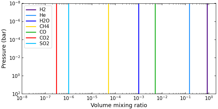
This example configuration file below computes free-VMR profiles with H₂ and He as filler gasses. The vmr_vars key defines one model per row (H₂O and CH⁴), where the first field is the model name and the second field its parameter value(s):

bulk = H2 He
vmr_vars =
    log_H2O  -3.0
    log_CH4  -4.3

Copy this file to your local folder. Then you can generate VMR profiles with the Python script below:

import matplotlib.pyplot as plt
import pyratbay as pb
import pyratbay.plots as pp
plt.ion()

# Generate a free-chemistry atmosphere
atm = pb.run("vmr_profile_free_constant.cfg")

# Plot the results
plt.figure(12, figsize=(7, 3.5))
plt.clf()
plt.subplots_adjust(0.1, 0.14, 0.99, 0.97)
ax = pp.abundance(
    atm.vmr, atm.press, atm.species,
    colors='default', xlim=[1e-8, 2.0], ax=plt.subplot(111),
)

And the results should look like this:

Non-isobaric VMR

The slant_X (non-isobaric) model consist of a slanted $\log {\rm VMR}$-$\log p$ profile, capped between two VMR values. The model has five free parameters, as described below:

Parameter	Description
`slope`	Slope of VMR profile: ${\rm d}(\log {\rm VMR}) / {\rm d}(\log p)$
`log_VMR0`	Reference VMR value at reference pressure `log_p0`
`log_p0`	Reference pressure level
`max_log_VMR`	Minimum VMR value (VMR profile is capped)
`min_log_VMR`	Maximum VMR value (VMR profile is capped)

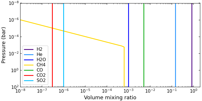
The example configuration file below computes free-VMR profiles with H₂ and He as filler gasses. The vmr_vars key defines the VMR models. Each row defines which model (here, a non-isobaric CH⁴ profile and a constant H₂O profile), followed by the model parameters:

bulk = H2 He

# slant params: slope  VMR0  p0   min   max
vmr_vars =
    slant_CH4   1.5  -3.5  -3.0  -inf  -3.2
    log_H2O    -3.0

Click here to show/hide: vmr_profile_free_non_isobaric.cfg

File: vmr_profile_free_non_isobaric.cfg¶

[pyrat]
# Pyrat Bay run mode: [tli atmosphere spectrum opacity retrieval radeq]
runmode = atmosphere

# Output file name and verbosity
logfile = WASP80b_free_chemistry_atmosphere.log
verb = 2

# Pressure profile
ptop = 1.0e-8 bar
pbottom = 100.0 bar
nlayers = 81

# Temperature profile [isothermal guillot madhu]
tmodel = isothermal
tpars = 850.0

# Chemistry model
chemistry = free
species =       H2     He   H2O   CH4    CO   CO2   SO2
uniform_vmr = 0.85  0.149  4e-3  1e-5  5e-3  3e-7  1e-6

bulk = H2 He
# slant models m    VMR0   p0    min      max
vmr_vars =
    log_H2O    -3.0
    slant_CH4   1.5  -3.5  -3.0  -inf  -3.2

Copy this file to your local folder. Then you can generate VMR profiles with the Python script below:

import matplotlib.pyplot as plt
import pyratbay as pb
import pyratbay.plots as pp
plt.ion()

# Generate a free-chemistry atmosphere
atm = pb.run("vmr_profile_free_non_isobaric.cfg")

# Plot the results
plt.figure(12, figsize=(7, 3.5))
plt.clf()
plt.subplots_adjust(0.1, 0.14, 0.99, 0.97)
ax = pp.abundance(
    atm.vmr, atm.press, atm.species,
    colors='default', xlim=[1e-8, 2.0], ax=plt.subplot(111),
)

And the results should look like this:

Note

While 5 parameters sounds like a lot, the advantage of this model is its flexibility. It can reproduce a range of constant, slanted, and slanted+constant profiles. See the examples in the figure below. In most cases, not all 5 parameters are relevant (this is particularly important for retrieval runs).

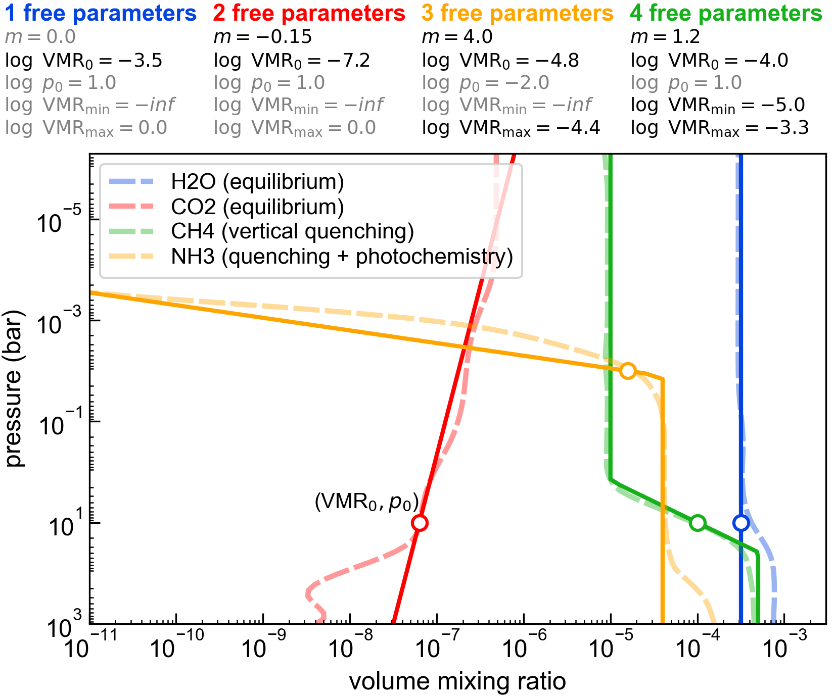
_images/non_isobaric_vmr_model.png — **Caption:** `slant_x` models for a variety of profiles from [Moses2011]¶

More Examples:

Equilibrium VMRs

Equilibrium calculations take heritage from the TEA package [Blecic2016], allowing users to select the set of atmospheric species, computing thermochemical equilibrium abundances via a Gibbs minimization (given the elemental composition, and pressure-temperature profile).

An equilibrium run must set chemistry = equilibrium in the configuration file, and define the set of species present in the atmosphere via the species key. For example, for a SCHON chemistry:

# Chemistry model and composition [free equilibrium]
chemistry = equilibrium
species =
    H2  He  H  H2O  CH4  CO  CO2  HCN  NH3  N2  OH  C2H2
    S2  SH  H2S  SO2  SO  OCS  CS  CS2

The equilibrium calculation assumes a solar elemental composition from [Asplund2021] as starting point. These elemental abundances can be further customized in a variety of ways via the vmr_vars key. The table below shows the available options:

`vmr_vars`	Description	Comments
`[M/H]`	Global metallicity scale factor for all metal elements (i.e., everything except H and He)	dex units relative to solar.
`[X/H]`	Metallicity scale factor for element `X` (for example `[C/H]` or `[O/H]`)	dex units relative to solar. Note this overrides `[M/H]` for element `X`
`X/Y`	Set abundance of element `X` relative to element `Y` (for example `C/O` ratio)	Note this overrides `[M/H]` for `X`, but `Y` can be previously scaled by `[M/H]` or `[Y/H]`

Note

Note that users can use and combine as many VMR parameters as desired!

Examples

This sample configuration file computes equilibrium VMRs, scaling the abundances of carbon, oxygen, and all other metals.

Click here to show/hide: vmr_profile_equilibrium.cfg

File: vmr_profile_equilibrium.cfg¶

[pyrat]
# Pyrat Bay run mode: [tli atmosphere spectrum opacity retrieval radeq]
runmode = atmosphere

# Output file name and verbosity
logfile = WASP18b_equilibrium_atmosphere.log
verb = 2

# Pressure profile
ptop = 1.0e-8 bar
pbottom = 100.0 bar
nlayers = 81

# Temperature profile [isothermal guillot madhu]
tmodel = isothermal
tpars = 3000.0

# Chemistry model and composition [free equilibrium]
chemistry = equilibrium
species =
    H  He  C  N  O  F  Na  Mg  Al Si  P  S  Cl K  Ca  Ti  V Fe
    H2  H2O  CH4  CO  CO2  HCN  NH3  N2  OH  C2H2  C2H4
    S2  SH  H2S  SO2  SO  TiO  VO  TiO2  VO2   SiO  SiH  SiS  SiH4
    OCS PH PH3 PN PO KOH CS CS2 NaH  NaCl  HCl  KCl CaH  HF  AlF  NaOH
    e-  H-  H+  H2+  He+  Na-  Na+  Mg+ K-  K+  Fe+  Ti+  V+ SiH+ Si- Si+

# Scale independently the elemental abundances of carbon, oxygen, and
# all other metals (dex units, relative to solar)
vmr_vars =
    [M/H] 0.5
    [C/H] 0.7
    [O/H] 0.5

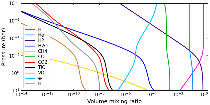
Copy this file to your local folder. Then you can generate VMR profiles with the Python script below:

import numpy as np
import matplotlib.pyplot as plt
plt.ion()

import pyratbay as pb
import pyratbay.plots as pp

# Compute a thermochemical-equilibrium atmosphere
atm = pb.run("vmr_profile_equilibrium.cfg")

# Only show molecules of interest
mol_show = ['H2', 'He', 'H', 'H-', 'e-', 'H2O', 'CO', 'CO2', 'CH4', 'TiO', 'VO']
imol = np.isin(atm.species, mol_show)

plt.figure(12, figsize=(7, 3.5))
plt.clf()
plt.subplots_adjust(0.1, 0.14, 0.99, 0.97)
ax = pp.abundance(
    atm.vmr[:,imol], atm.press, atm.species[imol],
    colors='default', xlim=[1e-14, 2.0], ax=plt.subplot(111),
)

And the results should look like this:

More Examples:

Equilibrium chemistry VMRs used in retrieval

Hybrid VMRs

Pyrat Bay also enables hybrid-chemistry calculations that embed free VMR profiles into an equilibrium-chemistry atmosphere. A hybrid-chemistry run must set chemistry = equilibrium in the configuration file, and define the set of species present in the atmosphere via the species key.

As for the equilibrium mode, the vmr_vars key allows one to customize the elemental composition, except that now users can include free VMR profiles with the log_X option:

`vmr_vars`	Description	Comments
`[M/H]`	Global metallicity scale factor for all metal elements (i.e., everything except H and He)	dex units relative to solar.
`[X/H]`	Metallicity scale factor for element `X` (for example `[C/H]` or `[O/H]`)	dex units relative to solar. Note this overrides `[M/H]` for element `X`
`X/Y`	Set abundance of element `X` relative to element `Y` (for example `C/O` ratio)	Note this overrides `[M/H]` for `X`, but `Y` can be previously scaled by `[M/H]` or `[Y/H]`
`log_X`	Constant with altitude VMR of species `X` (for example, `log_H2O`)	The VMR profile for species `X` is taken out of equilibrium

Note

In hybrid-chemistry runs, first all equilibrium variables will define the equilibrium-chemistry composition. Then, the log_X variables (if any) will override the abundance of the X species, taking them out of equilibrium, without altering any other abundance.

Examples

Click here to show/hide: vmr_profile_hybrid.cfg

File: vmr_profile_hybrid.cfg¶

[pyrat]
# Pyrat Bay run mode: [tli atmosphere spectrum opacity retrieval radeq]
runmode = atmosphere

# Output file name and verbosity
logfile = WASP39b_hybrid_atmosphere.log
verb = 2

# Pressure profile
ptop = 1.0e-8 bar
pbottom = 100.0 bar
nlayers = 81

# Temperature profile [isothermal guillot madhu]
tmodel = isothermal
tpars = 900.0

# Chemistry model and composition [free equilibrium]
chemistry = equilibrium
species =
    H  He  C  N  O  F  Na  Mg  Si  S  K  Ti  V Fe
    H2  H2O  CH4  CO  CO2  HCN  NH3  N2  OH  C2H2  C2H4 OCS CS CS2
    S2  SH  H2S  SO2  SO  TiO  VO  TiO2  VO2   SiO  SiH  SiS  SiH4
    e-  H-  H+  H2+  He+  Na-  Na+  Mg+ K-  K+  Fe+  Ti+  V+ SiH+ Si- Si+

# Scale independently the elemental abundances of carbon, oxygen, and
# all other metals (dex units, relative to solar)
vmr_vars =
    [M/H]     1.0
    [C/H]     0.8
    [O/H]     1.1
    log_SO2  -5.0

This configuration file computes a hybrid atmosphere in equilibrium for all species except SO₂, which is set to a constant VMR abundance (with a much larger than that expected in equilibrium):

# Chemistry model and composition [free equilibrium]
chemistry = equilibrium
species =
    H  He  C  N  O  F  Na  Mg  Si  S  K  Ti  V Fe
    H2  H2O  CH4  CO  CO2  HCN  NH3  N2  OH  C2H2  C2H4 OCS CS CS2
    S2  SH  H2S  SO2  SO  TiO  VO  TiO2  VO2   SiO  SiH  SiS  SiH4
    e-  H-  H+  H2+  He+  Na-  Na+  Mg+ K-  K+  Fe+  Ti+  V+ SiH+ Si- Si+

# Scale elemental abundances of carbon, oxygen, and metals.
# Then, adopt an out-of-equilibrium SO2 profile
vmr_vars =
    [M/H]    1.0
    [C/H]    0.8
    [O/H]    1.1
    log_SO2 -5.0

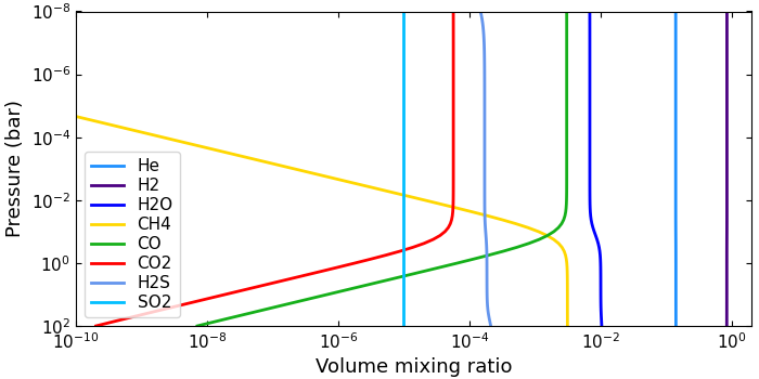
Copy this file to your local folder. Then you can generate VMR profiles with the Python script below:

import numpy as np
import pyratbay as pb
import pyratbay.plots as pp
import matplotlib.pyplot as plt
plt.ion()

# Compute a thermochemical-equilibrium atmosphere
atm = pb.run("vmr_profile_hybrid.cfg")

# Only show molecules of interest
mol_show = ['H2', 'He', 'H2O', 'CO', 'CO2', 'CH4', 'H2S', 'SO2']
imol = np.isin(atm.species, mol_show)

plt.figure(12, figsize=(7, 3.5))
plt.clf()
plt.subplots_adjust(0.1, 0.14, 0.99, 0.97)
ax = pp.abundance(
    atm.vmr[:,imol], atm.press, atm.species[imol],
    colors='default', xlim=[1e-10, 2.0], ax=plt.subplot(111),
)

And the results should look like this:

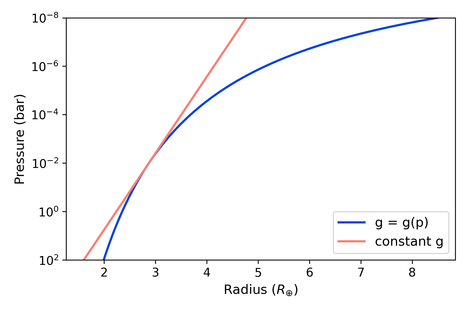
Radius¶

Setting the radmodel key signals the code to compute the radius profile (altitude of each pressure layer) assuming hydrostatic equilibrium and ideal gas law. There are two options, a pressure-dependent gravity model (radmodel=hydro_m, recommended):

\[\frac{dr}{r^2} = -\frac{k_{\rm B}T}{\mu G M_p} \frac{dp}{p},\]

or a constant-gravity model (radmodel=hydro_g):

\[dr = -\frac{k_{\rm B}T}{\mu g} \frac{dp}{p},\]

where $k_{\rm B}$ and $G$ are the Boltzmann and gravitational constants, respectively. $M_{\rm p}$ is the mass of the planet, defined by the user (for example, mplanet = 2.9 mearth). $T(p)$ and $\mu(p)$ are the atmospheric temperature and mean molecular mass profiles.

To solve the hydrostatic-equilibrium equation, users also need to provide a radius–pressure reference point, defining the condition $r(p_0) = R_0$. The rplanet and refpressure keys set $R_0$ and $p_0$, respectively.

Note

Note that the choice of the $\{p_0,R_0\}$ pair is somewhat arbitrary. A good practice is to choose values close to the transit radius of the planet. Although the pressure at the transit radius is a priori unknown for a give particular case [Griffith2014], its value lies at around 0.1 bar.

Examples¶

Here is an example of a hydrostatic-equilibrium atmosphere configuration file:

Click here to show/hide: profile_hydro_m.cfg

File: profile_hydro_m.cfg¶

[pyrat]

# Pyrat Bay run mode: [tli atmosphere spectrum opacity retrieval radeq]
runmode = atmosphere

# Log output (also atmospheric file output if output_atmfile is undefined):
logfile = Kepler_11c.log

# Pressure at the top and bottom of the atmosphere, and number of layers:
ptop = 1.0e-8 bar
pbottom = 100.0 bar
nlayers = 81

# Temperature-profile model, select from [isothermal guillot madhu]
tmodel = isothermal
tpars = 850.0

# Chemistry model [free equilibrium]
chemistry = free
species =       H2    He   Na  H2O  CH4   CO  CO2  NH3  HCN   N2
uniform_vmr = 0.85 0.149 5e-6 2e-3 1e-4 5e-4 1e-6 1e-5 1e-9 2e-4

# Altitude/radius profile model, select from [hydro_m, hydro_g]:
radmodel = hydro_m
rplanet = 2.87 rearth
mplanet = 2.86 mearth
refpressure = 0.01 bar

# Verbosity level (<0:errors, 0:warnings, 1:headlines, 2:details, 3:debug):
verb = 2

Click here to show/hide: profile_hydro_g.cfg

File: profile_hydro_g.cfg¶

[pyrat]

# Pyrat Bay run mode: [tli atmosphere spectrum opacity retrieval radeq]
runmode = atmosphere

# Log output (also atmospheric file output if output_atmfile is undefined):
logfile = Kepler_11c.log

# Pressure at the top and bottom of the atmosphere, and number of layers:
ptop = 1.0e-8 bar
pbottom = 100.0 bar
nlayers = 81

# Temperature-profile model, select from [isothermal guillot madhu]
tmodel = isothermal
tpars = 850.0

# Chemistry model [free equilibrium]
chemistry = free
species =       H2    He   Na  H2O  CH4   CO  CO2  NH3  HCN   N2
uniform_vmr = 0.85 0.149 5e-6 2e-3 1e-4 5e-4 1e-6 1e-5 1e-9 2e-4

# Altitude/radius profile model, select from [hydro_m, hydro_g]:
radmodel = hydro_g
rplanet = 2.87 rearth
mplanet = 2.86 mearth
refpressure = 0.01 bar

# Verbosity level (<0:errors, 0:warnings, 1:headlines, 2:details, 3:debug):
verb = 2

The following Python script creates and plots the profiles for the configuration file shown above:

import matplotlib.pyplot as plt
plt.ion()
import pyratbay as pb
import pyratbay.constants as pc

# A planet with Kepler-11c mass and radius:
atm = pb.run("profile_hydro_m.cfg")
atm_g = pb.run("profile_hydro_g.cfg")

# Plot the results:
plt.figure(12, figsize=(6,4))
plt.clf()
ax = plt.subplot(111)
ax.semilogy(atm.radius/pc.rearth, atm.press, lw=2, c='xkcd:blue', label='g = g(p)')
ax.semilogy(atm_g.radius/pc.rearth, atm_g.press, lw=2, c='salmon', label='constant g')
ax.set_ylim(1e2, 1e-8)
ax.set_xlabel(r'Radius $(R_{\oplus})$', fontsize=12)
ax.set_ylabel('Pressure (bar)', fontsize=12)
ax.tick_params(labelsize=11)
ax.legend(loc='lower right', fontsize=12)
plt.tight_layout()

And the results should look like this:

_images/pyrat_hydrostatic_equilibrium.png

`vmr_vars`	Description	Comments
`log_X`	Constant with altitude VMR of species `X` (for example, `log_H2O`)	Set \(\log_{10}({\rm VMR})\) of species `X`
`slant_X`	Non-isobaric VMR profile for species `X` (for example `slant_CH4`)	A 5-parameter model that allows for non-constant VMR profiles