Alkali opacity tutorial
This tutorial shows how to create Alkali opacity objects and compute their extinction coefficient spectra for a given atmospheric profile.
Note
You can also find this tutorial as a Python script here or as a jupyter notebook here.
[1]:
# Lets start by importing some necessary modules:
import pyratbay.atmosphere as pa
import pyratbay.constants as pc
import pyratbay.opacity as op
import pyratbay.spectrum as ps

import matplotlib.pyplot as plt
import numpy as np
Initialization
We will sample the models over a wavelength array and over an atmospheric profile. Lets create these first:
[2]:
# We will sample the opacity over a constant-resolution wavelength array
# (values have micron units)
wl_min = 0.5
wl_max = 1.0
resolution = 30000.0
wl = ps.constant_resolution_spectrum(wl_min, wl_max, resolution)

# Atmospheric pressure profile in bars:
nlayers = 81
pressure = pa.pressure('1e-8 bar', '1e2 bar', nlayers)

# Initialize a Na model:
sodium = op.alkali.SodiumVdW(pressure, wl=wl)
[3]:
# A print() call shows some useful info about the object
print(sodium)
Model name (name): 'sodium_vdw'
Model species (species): Na
Species mass (mass, amu): 22.989769
Profile hard cutoff from line center (cutoff, cm-1): 4500.0
Detuning parameter (detuning): 30.0
Lorentz-width parameter (lpar): 0.071
Partition function (Z): 2.0
Wavenumber  Wavelength          gf   Lower-state energy
      cm-1          um               cm-1
      (wn)                    (gf)   (elow)
  16960.87    0.589592   6.546e-01   0.000e+00
  16978.07    0.588995   1.309e+00   0.000e+00
Wavenumber (wn, cm-1):
   [20000.00 19999.33 19998.67 ... 10000.81 10000.47 10000.14]
Pressure (pressure, bar):
[1.000e-08 1.334e-08 1.778e-08 2.371e-08 3.162e-08 4.217e-08 5.623e-08
 7.499e-08 1.000e-07 1.334e-07 1.778e-07 2.371e-07 3.162e-07 4.217e-07
 5.623e-07 7.499e-07 1.000e-06 1.334e-06 1.778e-06 2.371e-06 3.162e-06
 4.217e-06 5.623e-06 7.499e-06 1.000e-05 1.334e-05 1.778e-05 2.371e-05
 3.162e-05 4.217e-05 5.623e-05 7.499e-05 1.000e-04 1.334e-04 1.778e-04
 2.371e-04 3.162e-04 4.217e-04 5.623e-04 7.499e-04 1.000e-03 1.334e-03
 1.778e-03 2.371e-03 3.162e-03 4.217e-03 5.623e-03 7.499e-03 1.000e-02
 1.334e-02 1.778e-02 2.371e-02 3.162e-02 4.217e-02 5.623e-02 7.499e-02
 1.000e-01 1.334e-01 1.778e-01 2.371e-01 3.162e-01 4.217e-01 5.623e-01
 7.499e-01 1.000e+00 1.334e+00 1.778e+00 2.371e+00 3.162e+00 4.217e+00
 5.623e+00 7.499e+00 1.000e+01 1.334e+01 1.778e+01 2.371e+01 3.162e+01
 4.217e+01 5.623e+01 7.499e+01 1.000e+02]
Cross section (cross_section, cm2 molecule-1):
None
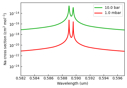
[4]:
# Evaluate the cross_section over an isothermal profile
temperature = np.tile(1800.0, nlayers)
Na_cross_section = sodium.calc_cross_section(temperature)


# Show the spectra at a couple of layers
fig = plt.figure(2)
fig.set_size_inches(5.0, 3.5)
plt.clf()
ax = plt.subplot(111)
ax.plot(wl, Na_cross_section[72], color='xkcd:green', lw=2.0, label='10.0 bar')
ax.plot(wl, Na_cross_section[40], color='red', lw=2.0, label='1.0 mbar')
ax.set_yscale('log')
ax.set_xlabel('Wavelength (um)')
ax.set_xlim(np.amin(wl), np.amax(wl))
ax.set_xlim(0.582, 0.597)
ax.tick_params(which='both', direction='in')
ax.set_ylabel('Na cross section (cm$^{2}$ mol$^{-1}$)')
ax.legend(loc='upper right')
plt.tight_layout()
Extinction coefficient
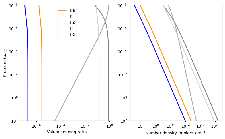
For radiative-transfer calculations we need the extinction coefficient, for which we need first number density profiles of the species. Here we first simulate a simple atmosphere in thermochemical equilibrium to compute the number densities under the ideal gas law:
[5]:
# A very simple atmosphere with solar abundance in thermochemical equilibrium
species = ['Na', 'K', 'H2', 'H', 'He']
net = pa.chemistry('tea', pressure, temperature, species)
# Number-density profiles under IGL (molecules per cm3)
number_densities = pa.ideal_gas_density(net.vmr, pressure, temperature)

Na_number_density = number_densities[:,0]
K_number_density = number_densities[:,1]


# Show profiles:
cols = ['darkorange', 'blue', 'gray', 'darkgray', 'lightgray']
plt.figure(1, (8,5))
plt.clf()
ax = plt.subplot(121)
for i, spec in enumerate(species):
    ax.plot(net.vmr[:,i], pressure, color=cols[i], lw=2.0, label=spec)
ax.set_xscale('log')
ax.set_yscale('log')
ax.set_ylim(100, 1e-8)
ax.set_xlabel('Volume mixing ratio')
ax.set_ylabel('Pressure (bar)')
ax.legend(loc='best')

ax = plt.subplot(122)
for i, spec in enumerate(species):
    ax.plot(number_densities[:,i], pressure, color=cols[i], lw=2.0, label=spec)
ax.set_xscale('log')
ax.set_yscale('log')
ax.set_ylim(100, 1e-8)
ax.set_xlabel('Number density (molecs cm$^{-3}$)')
plt.tight_layout()
Compute chemical abundances.
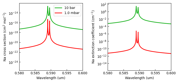
[6]:
# Extinction-coefficient over the atmospheric profile
Na_extinction = sodium.calc_extinction_coefficient(
    temperature,
    Na_number_density,
)


# Show the spectra at a couple of layers
fig = plt.figure(2)
fig.set_size_inches(7.5, 3.5)
plt.clf()
ax = plt.subplot(121)
ax.plot(wl, sodium.cross_section[72], color='xkcd:green', lw=2.0, label='10 bar')
ax.plot(wl, sodium.cross_section[40], color='red', lw=2.0, label='1.0 mbar')
ax.set_yscale('log')
ax.set_xlabel('Wavelength (um)')
ax.set_xlim(np.amin(wl), np.amax(wl))
ax.set_xlim(0.58, 0.60)
ax.tick_params(which='both', direction='in')
ax.set_ylabel('Na cross section (cm$^{2}$ mol$^{-1}$)')
ax.legend(loc='upper right')

ax = plt.subplot(122)
ax.plot(wl, Na_extinction[72], color='xkcd:green', lw=2.0)
ax.plot(wl, Na_extinction[40], color='red', lw=2.0)
ax.set_yscale('log')
ax.set_xlabel('Wavelength (um)')
ax.set_xlim(np.amin(wl), np.amax(wl))
ax.set_xlim(0.58, 0.60)
ax.tick_params(which='both', direction='in')
ax.set_ylabel('Na extinction coefficient (cm$^{-1}$)')
plt.tight_layout()
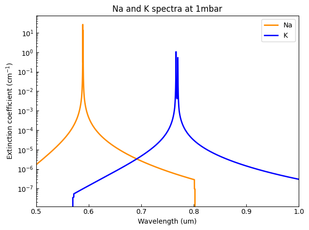
Sodium and Potassium models
[7]:
# Similarly, we can compute K extinction coefficients
potassium = op.alkali.PotassiumVdW(pressure, wl=wl)
K_extinction = potassium.calc_extinction_coefficient(
    temperature, K_number_density,
)

# Plot K extinction along Na's
fig = plt.figure(3)
plt.clf()
ax = plt.subplot(111)
ax.plot(wl, Na_extinction[72], color='darkorange', lw=2.0, label='Na')
ax.plot(wl, K_extinction[72], color='blue', lw=2.0, label='K')
ax.set_yscale('log')
ax.set_xlabel('Wavelength (um)')
ax.set_xlim(np.amin(wl), np.amax(wl))
ax.set_xlim(0.5, 1.0)
ax.tick_params(which='both', direction='in')
ax.set_ylabel('Extinction coefficient (cm$^{-1}$)')
ax.legend(loc='upper right')
ax.set_title('Na and K spectra at 1mbar')
plt.tight_layout()
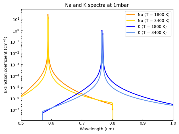
[8]:
# To evaulate under new atmospheric conditions, simply call the
# extinction_coefficient() method with the new values:

# A hotter atmosphere
temp_hot = np.tile(3400.0, nlayers)
vmr_hot = net.thermochemical_equilibrium(temperature=temp_hot)
density_hot = pa.ideal_gas_density(vmr_hot, pressure, temp_hot)
Na_density_hot = density_hot[:,0]
K_density_hot = density_hot[:,1]

# New opacities
Na_extinction_hot = sodium.calc_extinction_coefficient(
    temp_hot, Na_density_hot,
)
K_extinction_hot = potassium.calc_extinction_coefficient(
    temp_hot, K_density_hot,
)


# Plot Na and K opacities
fig = plt.figure(4)
plt.clf()
ax = plt.subplot(111)
ax.plot(wl, Na_extinction[72], color='darkorange', lw=2.0, label='Na (T = 1800 K)')
ax.plot(wl, Na_extinction_hot[72], color='gold', lw=2.0, label='Na (T = 3400 K)')
ax.plot(wl, K_extinction[72], color='blue', lw=2.0, label='K (T = 1800 K)')
ax.plot(wl, K_extinction_hot[72], color='cornflowerblue', lw=2.0, label='K (T = 3400 K)')
ax.set_yscale('log')
ax.set_xlabel('Wavelength (um)')
ax.set_xlim(np.amin(wl), np.amax(wl))
ax.set_xlim(0.5, 1.0)
ax.tick_params(which='both', direction='in')
ax.set_ylabel('Extinction coefficient (cm$^{-1}$)')
ax.legend(loc='upper right')
ax.set_title('Na and K spectra at 1mbar')
plt.tight_layout()