Repack line sampling

Sometimes, computing cross-section spectra from billions of line transitions becomes unfeasible. For such cases, the repack tool [Cubillos2017b] helps to identify and retain the strong line transitions that dominate the spectrum. repack effectively the line list down to millions, without significantly impacting the cross section spectra. This tutorial shows how to fetch line lists that have been pre-processed with repack, and sample them into cross-section files for use in Pyrat Bay radiative-transfer calculations.

Pyrat Bay has a two-step process to process line lists:

1. Convert line lists from their original format (e.g., HITRAN .par files, ExoMol .states/.trans files) into transition-line information files (TLI files). This is simple a re-formatting step, the data is still kept as the info per line-transition (wavelengths, gf, Elow, isotope). TLI files can readily be used for Pyrat Bay radiative-transfer calculations, but such runs are slow as the code computes the lines shape and strength on the fly to obtain the cross sections.

2. Conver TLI files into cross-section tables (saved as Numpy .npz files). This step evaluates (i.e., samples) the line-transition information over a grid of [wavelength, temperature, pressure], which involves computing the line shape and strength of all lines at each given wl, pressure, and temperature value of the grid. Cross-section tables are ideal for radiative-transfer calculations, since the code simply interpolates from them (and therefore, these calculations are fast).

The main issue with cross-section is that they are not too flexible (one might want to change, e.g., the wavelength resolution or line broadening parameters, for which the user would need to re-generate cross-sections from the TLI files). For this reason Pyrat Bay was designed with this two-step approach.

---

Download Repack data

You can find ExoMol-repacked line lists from this Zenodo repository (DOI: 10.5281/zenodo.3768503):

• https://doi.org/10.5281/zenodo.3768503

The following table shows species already processed with repack and are ready for use:

Available linelists

Species/link	Database name	Isotopologues	References
H2O	pokazatel	116	[Polyansky2018]
CH4	mm	2111	[Yurchenko2024a]
CO2	ai3000k	266, 366, 628, 627	[Huang2023]
CO2	ucl4000	266	[Yurchenko2020]
NH3	coyute	4111, 5111	[Coles2019] [Yurchenko2024b]
TiO	toto	66, 76, 86, 96, 06	[McKemmish2019]
VO	hyvo	16	[Bowesman2024]
HCN	harris & larner	124, 134	[Harris2006] [Harris2008]
SO2	exoames	266	[Underwood2016]
H2S	ayt2	112	[Azzam2016] [Chubb2018]
C2H2	acety	2211	[Chubb2020]

For this demo, we will work with the VO repack line list. We fetch the data can do this with the following prompt commands:

# Download the data
wget https://zenodo.org/records/14266247/files/VO_exomol_hyvo_0.22-50um_100-3500K_threshold_0.01_lbl.dat
wget https://www.exomol.com/db/VO/51V-16O/HyVO/51V-16O__HyVO.pf

---

Format partition functions

Before generating the TLI file, we will format the partition-function files from ExoMol for use in Pyrat Bay. We can do this with the following prompt command where we first specify the source (exomol) and then list all ‘.pf’ files of interest (one can combine multiple isotopologues of a species into a single file):

From .pf files

If the ExoMol .pf files sample the temperature range of interest. Then use their .pf files directly:

pbay -pf exomol 51V-16O__HyVO.pf

From Exomol .states

Alternatively, if you expect to probe higher temperatures than those sample in the .pf files, the we can compute the partitions from the .states files with the command below. Here one specifies the temperature ranges and sampling step.

#             T_low  T_high  delta_T
pbay -pf states 5.0  10000.0  5.0  51V-16O__HyVO.states

This will produce the PF_exomol_VO.dat file, which can be passed as input for the TLI config file.

---

Compute TLI files

The easiest way to generate TLI files is via configuration files and the command line. The config file below converts the repack ExoMol/VO line-lists (see dblist) into a TLI file (see tlifile or logfile). The partition-function information must also be provided (see pflist).

Lastly, the user can specify the wavelength range of the extracted data (see wl_low and wl_high). Normally one want to the widest possible range (to avoid needing to re-calculating TLI files if a future calculation needs it), but for sake of this demo, we will extract just over a narrow region:

File: line_sample_repack_VO_tli.cfg

[pyrat]

# Pyrat Bay run mode: [tli atmosphere spectrum opacity retrieval radeq]
runmode = tli

# Output log and TLI file (if you ommit `tlifile`, it will be automatically generated from the logfile):
logfile = exomol_repack_VO_0.3-30.0um.log

# List of line-transtion databases:
dblist = VO_exomol_hyvo_0.22-50um_100-3500K_threshold_0.01_lbl.dat

# Type of line-transition database, select from:
# [hitran exomol repack]
dbtype = repack

# List of partition functions for each database:
pflist = PF_exomol_VO.dat

# Initial and final wavelength:
wl_low = 0.3 um
wl_high = 30.0 um

# Verbosity level [1--3]:
verb = 2

To generate the tli files, we run these Pyrat Bay prompt commands:

pbay -c line_sample_repack_VO_tli.cfg

---

Compute cross-section tables

As with TLI files, cross-section files can be generated via configuration files and the command line. The config file below computes a cross-section table (with the output name determined by the sampled_cross_sec or logfile parameters).

These parameters define each array of the cross-section table:

• The pbottom, ptop, and nlayers parameters define the pressure sampling array

• The tmin, tmax, and tstep parameters define the temperature sampling array

• The wl_low, wl_high, and resolution parameters define the spectral array at a constant resolution (alternatively, one can replace resolution with wnstep to sample at a constant \(\Delta \text{wavenumber}\), units in cm\(^{-1}\))

For the composition (species), make sure to include the molecule for which we are computing the cross-sections. Also, include the background gas, which is relevant for the pressure broadening (here, we assume a H2/He-dominated atmosphere). Only the VMR values of the background gasses are important, trace-gas VMRs are irrelevant (see chemistry or uniform_vmr. tmodel and tpars are needed to define the atmosphere’s temperature profile, but for an opacity run, these do not impact the calculations.

The optional voigt_extent and voigt_cutoff keys set the extent of the profiles wings from the line centers. voigt_extent sets the maximum extent in units of HWHM (default is 300 HWHM). voigt_cutoff sets the maximum extent in wavenumber units of cm^-1 (default is 25.0 cm^-1). For any given profile, the code truncates the line wing at the minimum value of either voigt_extent or voigt_cutoff.

Lastly, the user can set ncpu to speed up the calculations using parallel computing.

File: line_sample_repack_VO_opacity.cfg

[pyrat]

# Pyrat Bay run mode: [tli atmosphere spectrum opacity retrieval radeq]
runmode = opacity

# Output log and cross-section file:
# (if you ommit extfile it will be automatically generated from logfile name)
logfile = cross_section_R025K_0150-3000K_0.3-30.0um_exomol_VO_hyvo.log

# Input TLI file:
tlifile = exomol_repack_VO_0.3-30.0um.tli

# Pressure sampling:
pbottom = 100 bar
ptop = 1e-8 bar
nlayers = 51

# Temperature profile (needed, but not relevant for cross-section generation)
tmodel = isothermal
tpars = 1000.0

# A simplified H2/He-dominated composition
chemistry = free
species = H2  He  VO
uniform_vmr = 0.85 0.15 1e-4

# Wavelength sampling
wl_low = 0.3 um
wl_high = 30.0 um
resolution = 25000.0

# Extent of the Voigt profile wings (in HWHM and in cm-1, respectively):
#voigt_extent = 300.0
#voigt_cutoff = 25.0

# Cross-section temperature sampling:
tmin =  150
tmax = 3000
tstep = 150

# Number of CPUs for parallel processing:
ncpu = 16

# Verbosity level [1--3]
verb = 2

To generate the cross-section files, run this Pyrat Bay prompt command:

pbay -c line_sample_repack_VO_opacity.cfg

---

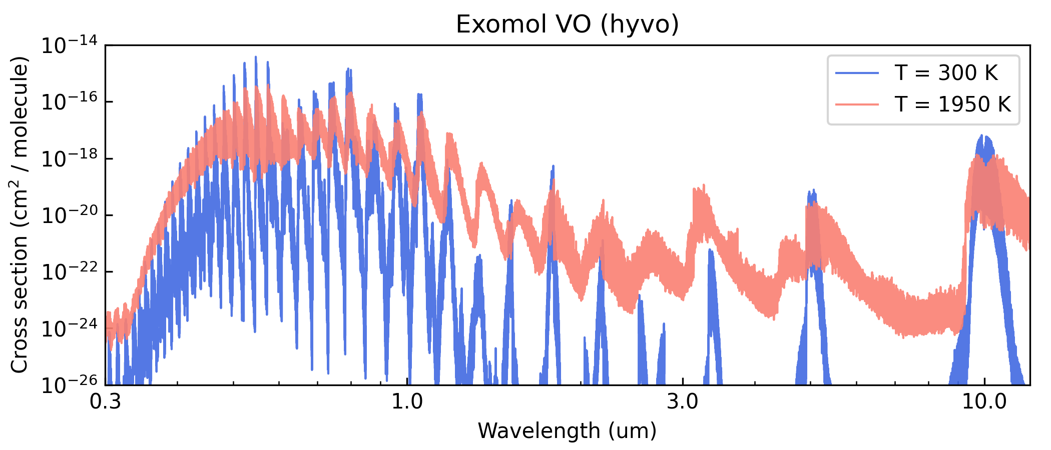
Here’s a Python script to take a look at the output cross section:

import pyratbay.io as io
import matplotlib
import matplotlib.pyplot as plt

cs_file = 'cross_section_R025K_0150-3000K_0.3-30.0um_exomol_VO_hyvo.npz'
units, mol, temp, press, wn, cross_section = io.read_opacity(cs_file)

p = 35
wl = 1e4/wn
colors = 'royalblue', 'salmon'

fig = plt.figure(0)
plt.clf()
fig.set_size_inches(7, 3)
plt.subplots_adjust(0.1, 0.145, 0.98, 0.9)
ax = plt.subplot(111)
for i,t in enumerate([1,12]):
    label = f'T = {temp[t]:.0f} K'
    plt.plot(
        wl, cross_section[t,p], lw=1.0,
        color=colors[i], alpha=0.9, label=label,
    )
plt.xscale('log')
plt.yscale('log')
ax.xaxis.set_minor_formatter(matplotlib.ticker.NullFormatter())
ax.xaxis.set_major_formatter(matplotlib.ticker.ScalarFormatter())
ax.set_xticks([0.3, 1.0, 3.0, 10.0])
plt.xlim(0.3, 12.0)
plt.ylim(1e-26, 1e-14)
plt.title('Exomol VO (hyvo)')
plt.xlabel('Wavelength (um)')
plt.ylabel(r'Cross section (cm$^{2}$ / molecule)')
plt.legend(loc='upper right')
ax.tick_params(which='both', direction='in')