Getting Started

The main goal of the Pyrat Bay package is to enable modeling of exoplanet atmospheres and their spectra. Since this involves several different physical processes, Pyrat Bay adopts a modular approach allowing the user to execute particular steps or concatenate multiple steps in a single run (see figure below).

_images/pyrat_user_case.png — `Pyrat Bay` use-case diagram and the main outputs from each case (italics). Solid arrows indicate steps that can be directly executed by the user. Dotted arrows indicate steps that can be linked in a single run.

The following table details what each of these steps do.

Run mode	Description
`tli`	Format line-by-line (LBL) opacity databases into a transition-line-information file (TLI, the format used by `Pyrat Bay` for spectral computations)
`atmosphere`	Generate a 1D atmospheric model (pressure, temperature, abundances, and altitude profiles)
`opacity`	Generate a cross-section table as function of wavenumber, temperature, pressure, and species
`spectrum`	Compute forward-modeling spectra (transmission or emission)
`mcmc`	Run an atmospheric retrieval

Any of these steps can be run either interactively though the Python Interpreter, or from the command line. To streamline execution, Pyrat Bay provides a single command to execute any of these runs. To set up any of these runs, Pyrat Bay uses configuration files following the standard INI format.

The Quick Example section below demonstrates a simple forward-modeling spectrum run, while the next sections give a thorough detail for each of the running modes. Finally, most of the low- and mid-level routines used for these calculations are available through the Pyrat Bay sub modules (see API).

System Requirements

Pyrat-Bay (version 1.0+) has been extensively tested to work on Unix/Linux and OS X machines, with the following software requirements:

Python >= 3.6
Numpy >= 1.8.1
Scipy >= 0.13.3
Matplotlib >= 1.3.1
Sympy >= 0.7.6
mc3 >= 3.0.7

Pyrat Bay may work with previous software versions; however, we do not guarantee nor provide support for that.

Install and Compile

To install Pyrat Bay run the following command from the terminal:

pip install pyratbay

Or if you prefer conda:

conda install -c conda-forge pyratbay

Alternatively (e.g., for developers), clone the repository to your local machine with the following terminal commands:

git clone --recursive https://github.com/pcubillos/pyratbay
cd pyratbay
python setup.py develop

Quick Example

The following script quickly you calculate a water transmission spectrum between 0.5 and 5.5 um. These instructions are meant to be executed from a Shell terminal. After you installed the package, create a working directory to place the files and execute the programs, e.g.:

mkdir run_demo
cd run_demo

Download the water line-transition database from the HITRAN server and unzip it:

# Using wget:
wget https://www.cfa.harvard.edu/HITRAN/HITRAN2012/HITRAN2012/By-Molecule/Compressed-files/01_hit12.zip
# Or alternatively: curl https://www.cfa.harvard.edu/HITRAN/HITRAN2012/HITRAN2012/By-Molecule/Compressed-files/01_hit12.zip -o 01_hit12.zip
unzip 01_hit12.zip

Copy the input and configuration files for the demo from the examples folder to your working directory. For example, use the following shell commands:

demo_path=https://raw.githubusercontent.com/pcubillos/pyratbay/master/examples/demo
wget $demo_path/demo_spectrum-emission.cfg
wget $demo_path/demo_spectrum-transmission.cfg
wget $demo_path/demo_tli-hitran.cfg
wget $demo_path/uniform.atm

Execute these commands from the shell to create a Transition-Line-Information (TLI) file, and then to use it to compute transmission and emission spectra:

# Format line-by-line opacity:
pbay -c demo_tli-hitran.cfg

# Compute transmission and emission spectra:
pbay -c demo_spectrum-transmission.cfg
pbay -c demo_spectrum-emission.cfg

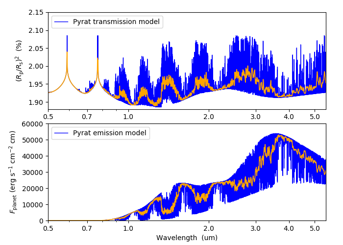
That’s it, now let’s see the results. The screen outputs and any warnings raised are saved into log files. The output spectrum is saved to a separate file, to see it, run this Python script (on interactive mode, I suggest starting the session with ipython --pylab):

import matplotlib
from scipy.ndimage.filters import gaussian_filter1d as gaussf
import matplotlib.pyplot as plt
plt.ion()

import pyratbay as pb
import pyratbay.io as io

wl, transmission = io.read_spectrum("./transmission_spectrum_demo.dat", wn=False)
wl, emission     = io.read_spectrum("./emission_spectrum_demo.dat", wn=False)

plt.figure(0, figsize=(7,5))
plt.clf()
plt.subplots_adjust(0.14, 0.1, 0.95, 0.95, hspace=0.15)
ax = plt.subplot(211)
plt.plot(wl, 100*transmission, "b", label="pyrat transmission model", lw=1.0)
plt.plot(wl, gaussf(100*transmission, sigma=5.0), "orange", lw=1.25)
plt.xscale('log')
plt.ylabel(r"$(R_{\rm p}/R_{\rm s})^2}$  (%)")
ax.get_xaxis().set_major_formatter(matplotlib.ticker.ScalarFormatter())
ax.set_xticks([0.5, 0.7, 1.0, 2.0, 3.0, 4.0, 5.0])
plt.xlim(0.5, 5.5)
plt.ylim(1.88, 2.15)
plt.legend(loc="upper left")

ax = plt.subplot(212)
plt.plot(wl, emission, "b", label="pyrat emission model", lw=1.0)
plt.plot(wl, gaussf(emission, sigma=5.0), "orange", lw=1.25)
plt.xscale('log')
plt.xlabel(r"Wavelength  (um)")
plt.ylabel(r"$F_{\rm planet}$ (erg s$^{-1}$ cm$^{-2}$ cm)")
ax.get_xaxis().set_major_formatter(matplotlib.ticker.ScalarFormatter())
ax.set_xticks([0.5, 0.7, 1.0, 2.0, 3.0, 4.0, 5.0])
plt.ylim(0, 60000)
plt.xlim(0.5, 5.5)
plt.legend(loc="upper left")
plt.draw()
plt.savefig("pyrat_spectrum_demo.pdf")

The output figure should look like this:

Command-line Run

As shown above, Pyrat Bay enables a command-line entry point to execute any of the runs listed above:

pbay -c config_file.cfg

The configuration file determines what run mode to execute by setting the runmode key. Each of these modes have different required/optional keys, which are detailed in further sections.

This same entry point offers a couple of secondary processes (display version, re-format files). To display these options, run:

pbay -h

Interactive Run

The same process can be executed from the Python Interpreter, after importing the Pyrat Bay package:

import pyratbay as pb
pyrat = pb.run('demo_spectrum-transmission.cfg')
ax = pyrat.plot_spectrum()

The output vary depending on the selected run mode. Additional low- and mid-level routines are also available through this package (see the API).

In the following sections you can find a more detailed description and examples of how to run Pyrat Bay for each available configuration.