Spectrum Tutorial

This run mode computes a transmission or emission spectrum, for a given atmospheric model.

Sample Configuration File

Here is a sample configuration file to compute a transmission spectrum (spectrum_transmission.cfg):

[pyrat]

# Pyrat Bay run mode, select from: [tli atmosphere spectrum opacity mcmc]
runmode = spectrum

# Output spectrum file:
specfile = ./transmission_spectrum_tutorial.dat

# Radiative-transer observing geometry, select from: [transit emission]
rt_path = transit

# Atmospheric model:
atmfile = WASP-00b.atm

# Wavelength sampling boundaries:
wllow  = 0.3 um
wlhigh = 5.0 um

# Wavenumber sampling rate and oversampling factor:
wnstep  = 1.0
wnosamp = 2160

# System parameters:
rstar = 1.27 rsun
tstar = 5800.0
smaxis = 0.045 au
mplanet = 0.6 mjup
rplanet = 1.0 rjup
tint = 100.0
# Reference pressure level at rplanet:
refpressure = 0.1 bar

# TLI opacity files:
tlifile = ./HITRAN_H2O_0.3-5.0um.tli

# Cross-section opacity files:
csfile =
    {ROOT}/pyratbay/data/CIA/CIA_Borysow_H2H2_0060-7000K_0.6-500um.dat
    {ROOT}/pyratbay/data/CIA/CIA_Borysow_H2He_0050-3000K_0.3-030um.dat

# Radius-profile model, select from: [hydro_m hydro_g]
radmodel = hydro_m

# Alkali models, select from: [sodium_vdw potassium_vdw]
alkali = sodium_vdw

# Rayleigh models, select from: [lecavelier dalgarno_H dalgarno_He dalgarno_H2]
rayleigh = lecavelier
rpars = 0.0 -4.0

# Cloud models, select from: [deck ccsgray]
clouds = deck
cpars = -0.5

# Number of CPUs for parallel processing:
ncpu = 7

# Maximum optical depth to calculate:
maxdepth = 10.0

# Verbosity level (<0:errors, 0:warnings, 1:headlines, 2:details, 3:debug):
verb = 2

# If defined, plot x-axis in log scale and set ticks at logxticks locations:
logxticks = 0.3 0.5 0.7 1.0 2.0 3.0 5.0

Observing Geometry

The rt_path key determines the radiative-transfer scheme and observing geometry. The following table list the available options:

`rt_path`	Observing geometry	Output spectrum	Units
transit	Transmission geometry	(\(R_{\rm p}\)/\(R_{\rm s}\))²	—
emission	Emission geometry	\(F_{\rm p}\)	erg s^-1 cm^-2 cm

For transmission geometry Pyrat Bay computes the transit depth, assuming parallel rays that travel from the star to the observer across the planetary atmosphere, which is composed of spherically symmetric shell layers. For emission geometry, Pyrat Bay computes the planetary flux emission spectrum, adopting the plane-parallel approximation, evaluating the emergent intensity at multiple angles with respect to the normal, and integrating the intensities over the planetary hemisphere. For more details, see [CubillosBlecic2021].

Atmospheric Model

The atmfile key sets the input atmospheric model from which to compute the spectrum. If the file pointed by atmfile does not exist, the codel will attempt to produce it (provided all necessary input parameters are set in the configuration file). The atmospheric model can be produced with Pyrat Bay or be a custom input from the user (as long as it follows the right format, see the API).

Spectrum Sampling

The wllow and wlhigh keys set the wavelength boundaries for the output spectrum (values must contain units; otherwise, set the units with the wlunits key). Alternatively, the user can set the spectrum boundaries by wavenumber using the wnlow and wnhigh keys (wavenumber keys are always in cm^-1; thus, the user should not provide units for them).

By default, the code produces an output spectrum at constant-wavenumber sampling rate. The wnstep sets the sampling rate in cm^-1. Note that this will be the output sampling rate. Internally, Pyrat Bay must compute line profiles at a higher resolution to ensure not to undersample the line profiles. The wnosamp key (an integer) sets the oversampling factor of the high-resolution sampling relative to wnstep (that is, the high-resolution sampling rate is wnstep/wnosamp). Typical values for the optical/IR are wnstep = 1.0 and wnosamp = 2000.

Alternatively, the user can request a constant-resolution output by setting the resolution key (where the resolution is \(R=\lambda/\Delta\lambda\)). Note that in this case, the configuration file must still define wnstep and wnosamp.

Voigt Profiles

To speed up calculations, Pyrat Bay pre-computes a grid of Voigt profiles at a fixed grid of Doppler and Lorentz half-width at half maximum (HWHM). When computing the LBL opacities, the code selects the closest profile to a given line, depending on the line properties.

The grid properties are set automatically by the code (based on the input atmosphere properties), so the user does not need to set them. However, these values can be set configuration file. The user can thus set the dmin, dmax, and ndop keys to set the ranges and number of samples for the Doppler HWHM array (in cm^-1 units). Similarly, the lmin, lmax, and nlor keys set the ranges and number of samples for the Lorentz HWHM array (in cm^-1 units).

Finally, the vextent and vcutoff keys set the Voigt profiles extent from the center of the line. vextent defines the maximum extent in units of HWHM (default is 100 HWHM), whereas vcutoff defines the maximum extent in units of cm^-1 (default is 25.0 cm^-1). For any given profile, the code truncates the line wing at the minimum value defined by vextent and vcutoff. A vcutoff value of zero results in no cutoff (vextent still applies though). Note that there are no known physical grounds that set the extent of a line profile. Typical (arbitrary) values found in the literature are on the order of ~100 HWHM and 25 cm^-1.

The range of HWHM values can vary strongly with pressure, temperature, or wavelength, in particular the Lorentz HWHM as it is inversely proportional to pressure. The following Figure, gives you an idea to set these values:

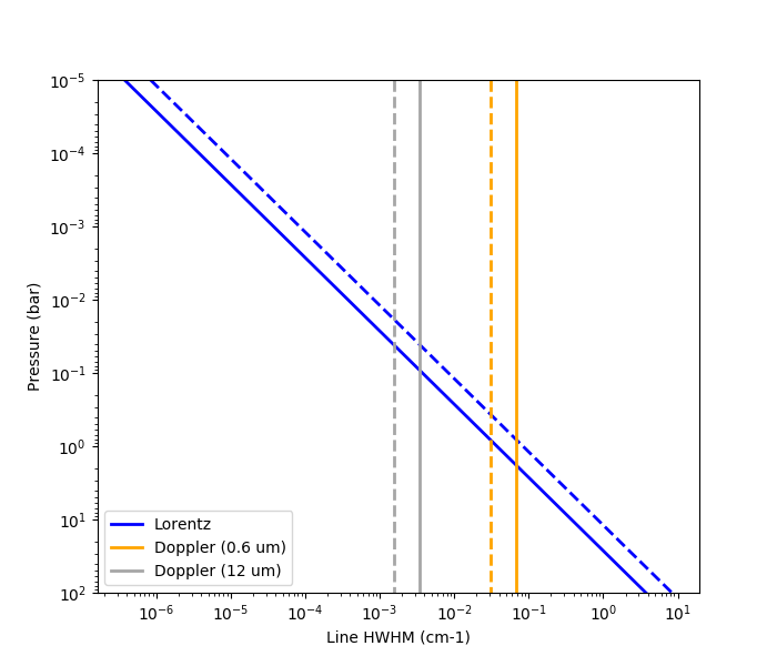
_images/broadening.png — HCN HWHM variation with pressure, temperature, and wavelength in a H₂-dominated atmosphere (see legend). Solid and dashed lines denote the HWHM at 2500 and 500 K, respectively ([Cubillos2017b]).

System Parameters

The system parameters have multiple uses.

Hill radius

The mstar, mplanet, and smaxis keys set the stellar mass, planetary mass, and orbital semi-major axis. If these keys are set in the configuration file, the code will compute the planetary Hill radius (\(R_{\rm H} = a \sqrt[3]{M_{\rm p}/3M_{\rm s}}\)). In such case, Pyrat Bay will neglect atmospheric layers at altitudes larger than \(R_{\rm H}\), since they should not be gravitationally bound to the planet.

Stellar spectrum

The tstar key sets the stellar effective temperature, which can be used to define a stellar blackbody spectrum (\(F_{\rm s}\), see Stellar Spectrum).

Radius Ratio

To compute eclipse depths from the emission spectra (\(F_{\rm p}\)), the user needs to set the rstar and rplanet keys, which define the stellar and planetary radius. The eclipse depths can then be computed as:

\[{\rm Eclipse\ depth} = \frac{F_{\rm p}}{F_{\rm s}} \left(\frac{R_{\rm p}}{R_{\rm s}}\right)^2\]

Line-by-line Opacities

Use the tlifile key to include TLI file(s) containing LBL opacities (to create a TLI file, see TLI Tutorial). The user can include zero, one, or multiple TLI files if desired.

Note that the tlifile opacities will be neglected if the configuration file sets input LBL opacities through the extfile (see the rules in Opacity Table as Input/output).

Cross-section Opacities

Use the csfile key to include opacities from cross-section files. A cross-section file contains opacity (in cm^-1 amagat^-2 units) tabulated as a function of temperature and wavenumber. Since this format is tabulated in wavenumber, it is best suited for opacities that vary smoothly with wavenumber, like collision-induced absorption (CIA). However, the code can also process LBL opacities, as long as the files follow the right format (more on this later).

The following table list the most-commonly used CIA opacity sources:

Sources	Species	T range	\(\nu\) range (cm^-1)	References
HITRAN	H₂–H₂	200–3000	1.0–500.0	[Richard2012] [Karman2019]
HITRAN	H₂–H	1000–2500	1.0–100.0	[Richard2012] [Karman2019]
HITRAN	H₂–He	200–9900	0.5–500.0	[Richard2012] [Karman2019]
Borysow	H₂–H₂	60–7000	0.6–500.0	[Borysow2001] [Borysow2002]
Borysow	H₂–He	50–3000	0.3–30.0	[Borysow1988] [Borysow1989a] [Borysow1989b]

Pyrat Bay provides commands to format the downloaded cross-section files from these databases.

For the HITRAN database, these commands re-format the downloaded CIA files and thins down the array (to reduce file size):

# Re-format HITRAN H2-H2 CIA file for Pyrat Bay:
# (last two arguments tell to take every 2nd and 10th temperature and wavenumber samples):
pbay -cs hitran H2-H2_2011.cia 2 10

# And for HITRAN H2-He CIA (taking every 4th and 10th temp and wavenumber samples):
pbay -cs hitran H2-He_2011.cia 4 10

For the Borysow database, the code provides already-formatted files for H₂-H₂ in the 60–7000K and 0.6–500 um range [here] (this file pieces together the tabulated H₂-H₂ files described in the references above); and for H₂-He in the 50–3500K and 0.3–100 um range [here] (this file was created using a re-implementation of the code described in the references above). The user can access these files via the {ROOT} shortcut, as in the example below:

csfile = {ROOT}/pyratbay/data/CIA/CIA_Borysow_H2H2_0060-7000K_0.6-500um.dat

Radius-profile Models

The radmodel key sets the model to compute the atmospheric layers’s altitude assuming hydrostatic equilibrium. This table shows the currently available models:

Models (`radmodel`)	Comments
hydro_m	Hydrostatic equilibrium with \(g(r)=GM/r^2\)
hydro_g	Hydrostatic equilibrium with constant gravity
[undefined]	Take radius profile from input atmospheric file if exists

See the Altitude Profiles section for details. The refpressure, rplanet, mplanet and gplanet keys set the planetary reference pressure and radius level (\(p_0\) and \(R_0\)), the planetary mass (\(M_p\)) and planetary surface gravity (\(g\)), respectively.

Note

Note that the user can supply its own atmospheric altitude profile (through the input atmospheric model), possibly not in hydrostatic equilibrium. In this case, do not set the radmodel key.

Alkali Opacity Models

Use the alkali key to include opacities from alkali species. Currently, the code provides the [Burrows2000] models for the sodium and potassium resonant lines, based on van der Waals and statistical theory. The following table lists the available alkali model names:

Models (`alkali`)	Species	References
sodium_vdw	Na	[Burrows2000]
potassium_vdw	K	[Burrows2000]

This implementation adopts the line parameters from the VALD database [Piskunov1995] and collisional-broadening half-width from [Iro2005].

Rayleigh Opacity Models

The rayleigh key sets Rayleigh opacity models. The following table lists the available Rayleigh model names:

Models (`rayleigh`)	Species	Parameters (`rpars`)	References
lecavelier	—	\(\log(f), \alpha\)	[Lecavelier2008]
dalgarno_H	H	—	[Dalgarno1962]
dalgarno_He	He	—	[Kurucz1970]
dalgarno_H2	H₂	—	[Kurucz1970]

The Dalgarno Rayleigh models are tailored for H, He, and H₂ species, and thus are not parametric. The Lecavelier Rayleigh model is more flexible and allows the user to modify the absorption strength and wavelength dependency according to:

\[k(\lambda) = f \kappa_0 \left(\frac{\lambda}{\lambda_0}\right)^\alpha,\]

where \(\lambda_0=0.35\) um and \(\kappa_0=5.31 \times 10^{-27}\) cm² molecule^-1 are constants, and \(\log(f)\) and \(\alpha\) are fitting parameters that can be set through the rpars key. Adopting values of \(\log(f)=0.0\) and \(\alpha=-4\) reduces the Rayleigh opacity to that expected for the H₂ molecule.

Note

Be aware that the implementation of the Lecavelier model uses the H₂ number-density profile (\(n_{\rm H2}\), in molecules cm^-3) to compute the extinction coefficient (in cm^-1 units) for a given atmospheric model: \(e(\lambda) = k(\lambda)\ n_{\rm H2}\). We do this, because we are mostly interested in H₂-dominated atmospheres, and most people consider a nearly constant H₂ profile. Obviously, this needs to be fixed at some point in the future for a more general use.

Cloud Opacity Models

Use the clouds key to include aerosol/haze/cloud opacities. Currently, the code provides simple gray cloud models (listed below), but soon we will include more complex Mie-scattering clouds for use in forward- and retrieval modeling. The following table lists the currently available cloud model names:

And these are the available haze/cloud models (clouds parameter):

Models (`clouds`)	Parameters (`cpars`)	Description
deck	\(\log(p_{\rm top})\)	Opaque gray cloud deck
ccsgray	\(\log(f)\), \(\log(p_{\rm t})\), \(\log(p_{\rm b})\)	Constant gray cross-section

Use the cpars key to set the cloud model parameters. The ‘deck’ model makes the atmosphere instantly opaque at/below the \(\log(p_{\rm top})\) pressure (in bar units).

The ‘ccsgray’ model creates a constant cross-section opacity between the \(p_{\rm t}\) and \(p_{\rm b}\) pressures (in bar units), and the \(\log(f)\) parameter scaling the opacity as: \(k = f\ k_0\), with \(\kappa_0=5.31 \times 10^{-27}\) cm² molecule^-1. This model uses the H₂ number-density profile to compute the extinction coefficient as: \(e(\lambda) = k\ n_{\rm H2}\) (in cm^-1 units). Since the H₂ mixing ratio is generally constant, the ‘ccsgray’ opacity will scale linearly with pressure over the atmosphere.

Patchy Cloud/Hazes

Set the fpatchy argument to compute transmission spectra from a linear combination of a clear and cloudy/hazy spectra. The cloudy/hazy component will include the opacity defined by the Cloud Opacity Models and the lecavelier Rayleigh Opacity Models. For example, for a 45% cloudy / 55% clear atmosphere, set:

# Patchy fraction, value between [0--1]:
fpatchy = 0.45

Temperature Models

The user can re-compute the temperature profile of the atmosphere by specifying the tmodel and tpars keys (see Temperature Profiles).

Abundances Scaling

Use the molmodel key to modify the abundance of certain atmospheric species (specified by molfree), according to the molpars key. The following table list the currently available models:

`molmodel`	Scaling	Description
vert	\(Q(p) = 10^X\)	Set abundance to given value
scale	\(Q(p) = Q_0(p)\ 10^X\)	Scale input abundance by given value

Here, the variable \(X\) represents the value in the molpars key, whereas \(Q_0\) is the abundance of the given species taken from the atmospheric file atmfile. Note that the user can specify as many scaling parameters as wished, as long as there are corresponding values for these three keys (molmodel, molfree, molpars).

To preserve the sum of the mixing fractions at 1.0 at each layer, the code will ‘adjust’ the values of certain ‘bulk’ species. The user needs to set these species through the bulk key. A good practice is to set here the dominant species in an atmosphere. If there is more than one ‘bulk’ species, the ratio of their abundances is preserved.

For example, the following configuration will set uniform mole mixing fractions for H₂O and CO of \(10^{-3}\) and \(10^{-4}\), respectively (regardless of input values); scale the input TiO profile by a factor of 10.0, and adjust the abundances of H₂ and He to preserve a total mixing fraction of 1.0 at each layer:

molmodel = vert  vert  scale
molfree  =  H2O    CO    TiO
molpars  = -3.0  -4.0   -1.0
bulk     = H2 He

Stellar Spectrum

Pyrat Bay provides several options to set a stellar spectrum. The stellar spectrum is required to compute eclipse depths as the planet-to-star flux spectrum. In order of precedence:

The starspec key sets the path to a custom spectrum file containing a spectrum. This file should contain in the first column the wavelength array in microns, and in the second column the flux spectrum in erg s^-1 cm^-2 cm units.

Alternatively, the user can use a Kurucz stellar model ([Castelli2003]) by setting the kurucz key to the path to a Kurucz model. These models can be downloaded from this link: http://kurucz.harvard.edu/grids/ In this case, the code selects the correct Kurucz model based on the stellar temperature (tstar key) and surface gravity (gstar key).

Finally, the user can set a blackbody stellar spectrum by setting the tstar key with the stellar effective temperature (in Kelvin units).

(MARCS and PHOENIX are TBI upon popular demand)

Filter Pass-bands

Use the filters key to set the path to instrument filter pass-bands (see [link to formats?]). These can be used to compute band-integrated values for the transmission or eclipse-depth spectra.

Observed Data

Use the data and uncert keys to set values for observed transit- or eclipse-depth values and their uncertainties, respectively. Logically, you want to set data values corresponding to the filters pass-bands.

Use the dunits key to specify the units of the data and uncert values (default: dunits = none). Typical values are: ‘none’, ‘percent’, or ‘ppm’ (see Units section).

Note

Note that the filters, data, and uncert keys are not strictly required for a spectrum run, but they will allow the code to plot these information if requested (see [link to plots]).

Other Configuration Parameters

Number of CPUs

The ncpu key sets the number of CPUs to use when computing LBL opacities or when running retrievals (default: ncpu = 1).

Verbosity

The verb key sets the screen-output and logfile verbosity level. Higher verb values will display increasingly levels of detail according to the following table:

`verb`	Screen Outputs
<0	Errors
0	Warnings
1	Headlines
2	Details
3	Debug

Log File

Use the logfile key to set a file name where to save the screen outputs (same content as the screen output). If this is not set by the user, the code will default the logfile to the output file of each corresponding runmode (changing the file extension to ‘.log’). The following table lists the files from where the code will take the default name for each runmode:

`runmode`	Default `logfile` name
tli	`tlifile`
atmosphere	`atmfile`
spectrum	`specfile`
opacity	`extfile`
mcmc	`mcmcfile`

Optical-depth Cutoff

The maxdepth key sets an optical-depth cutoff to stop the radiative-transfer calculations. Since there is little transmitted intensity through a layer when the optical depth is greater than one, layers where \(\tau \gg 1\) won’t impact on the resulting spectrum. The default value of maxdepth = 10.0 is thus an appropriate conservative value.

Plane-parallel Hemispheric Integration

For eclipse geometry, the code computes the emergent intensity under the plane-parallel approximation, and then it integrates (sums) intensity spectra at different angles with respect to the normal to model the emitted flux spectrum. The raygrid sets the angles (in degrees) where to evaluate these intensities (default: raygrid = 0 20 40 60 80). The user can set custom values for these angles as long as: (1) the first value is zero (normal to the planet’s ‘surface’), (2) they lie in the [0,90) range, and (3) they are increasing order.

Alternatively, the user can set the quadrature key to perform a Gaussian-quadrature integration, where the quadrature value sets number of Gaussian-quadrature points (in which case, raygrid will be ignored).

Examples

Note

Before running this example, make sure that you have generated the TLI file from the TLI Example, generated the atmospheric profiles from the Abundance-profile Examples, and download the configuration file shown above, e.g., with these shell commands:

tutorial_path=https://raw.githubusercontent.com/pcubillos/pyratbay/master/examples/tutorial
wget $tutorial_path/spectrum_transmission.cfg

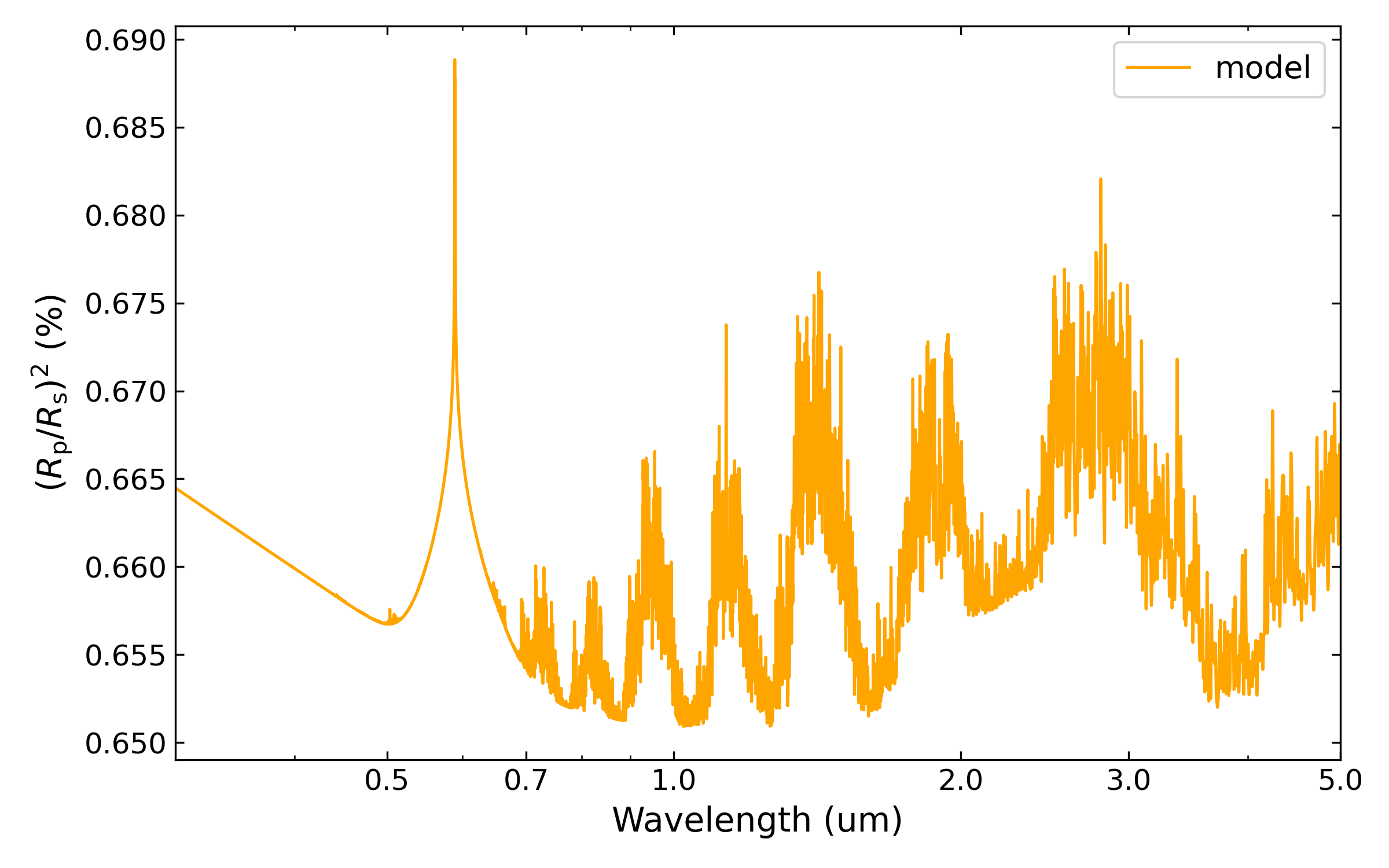
In an interactive run, a spectrum run returns a ‘pyrat’ object that contains all input, intermediate, and output variables used to compute the spectrum. The following Python script computes and plots a transmission spectrum using the configuration file found at the top of this tutorial:

import matplotlib.pyplot as plt
plt.ion()

import pyratbay as pb
import pyratbay.constants as pc

pyrat = pb.run('spectrum_transmission.cfg')

# Plot the resulting spectrum:
wl = 1.0 / (pyrat.spec.wn*pc.um)
depth = pyrat.spec.spectrum / pc.percent
wl_ticks = [0.3, 0.5, 0.7, 1.0, 2.0, 3.0, 5.0]

plt.figure(-3, (7,4))
plt.clf()
ax = plt.subplot(111)
plt.semilogx(wl, depth, "-", color='orange', lw=1.0)
ax.get_xaxis().set_major_formatter(matplotlib.ticker.ScalarFormatter())
ax.set_xticks(wl_ticks)
plt.xlim(0.3, 5.0)
plt.ylabel("Transit depth (Rp/Rs)$^2$ (%)")
plt.xlabel("Wavelength (um)")

# Or, alternatively:
ax = pyrat.plot_spectrum()

And the results should look like this:

_images/pyrat_transmission-spectrum_tutorial.png

Note

Note that although the user can define most input units, nearly all variables are stored in CGS units in the ‘pyrat’ object.

The ‘pyrat’ object is modular, and implements several convenience methods to plot and display its content, as in the following example:

# pyrat object's string representation:
print(pyrat)

# String representation of the spectral variables:
print(pyrat.spec)