Atmosphere Tutorial

This run mode generates a 1D atmospheric model (pressure, temperature, abundances, and altitude profiles), and saves it to a file. At minimum, the user needs to provide the arguments required to compute the pressure and temperature profiles. Further, Pyrat Bay will compute volume-mixing ratio (abundance) profiles only if the user sets the chemistry and respective arguments. Likewise, the code will compute the altitude profiles only if the user provides the radmodel and respective arguments (which also require that the abundance profiles to be defined).

Regardless of which profiles are computed, in an interactive run the code returns a five-element tuple containing the pressure profile (barye), the temperature profile (Kelvin), the abundance profiles (volume mixing fraction), the species names, and the altitude profile (cm). The outputs that were not calculated are set to None. Also, regardless of the input units, the output variables will always be in CGS units.

Pressure Profile

The pressure profile model is an equi-spaced array in log-pressure, determined by the pressure at the top of the atmosphere ptop, at the bottom of the atmosphere pbottom, and the number of layers nlayers.

The units for the ptop and pbottom pressures may be defined in-place along with the variable value (e.g., pbottom = 100 bar) or through the punits key (in-place units take precedence over punits). See Units for a list of available units.

Temperature Profiles

Currently, there are three temperature models (tmodel argument) to compute temperature profiles. Each one requires a different set of parameters (tpars), which is described in the table and sections below:

Models (`tmodel`)	Parameters (`tpars`)	References
isothermal	\(T_0\)	—
guillot	\(\log_{10}(\kappa')\), \(\log_{10}(\gamma_1)\), \(\log_{10}(\gamma_2)\), \(\alpha\), \(T_{\rm irr}\), \(T_{\rm int}\)	[Line2013]
madhu	\(\log_{10}(p_1)\), \(\log_{10}(p_2)\), \(\log_{10}(p_3)\), \(a_1\), \(a_2\), \(T_0\)	[Madhusudhan2009]

Isothemal profile

The isothermal model is the simplest model, having just one free parameter (tpars): the temperature (\(T_0\)) at all layers.

Here is an example of an isothermal atmosphere configuration file:

[pyrat]

# Pyrat Bay run mode, select from: [tli atmosphere spectrum opacity mcmc]
runmode = atmosphere

# Output atmospheric file:
atmfile = pt_isothermal_tutorial.atm

# Pressure at the top and bottom of the atmosphere, and number of layers:
ptop = 1.0e-6 bar
pbottom = 100.0 bar
nlayers = 100

# Temperature-profile model, select from [isothermal guillot madhu]
tmodel = isothermal
tpars = 990.0

# Verbosity level (<0:errors, 0:warnings, 1:headlines, 2:details, 3:debug):
verb = 2

Guillot profile

The guillot model has six parameters as defined in [Line2013]: \(\log_{10}(\kappa')\), \(\log_{10}(\gamma_1)\), \(\log_{10}(\gamma_2)\), \(\alpha\), \(T_{\rm irr}\) and \(T_{\rm int}\). The temperature profile is given as:

\[T^4(p) = \frac{3 T_{\rm int}^{4}}{4} \left(\frac{2}{3} + \tau\right) + (1-\alpha) \frac{3 T_{\rm irr}^{4}}{4} \xi_1(\tau) + \alpha \frac{3 T_{\rm irr}^{4}}{4} \xi_2(\tau),\]

with

\[\xi_i(\tau) = \frac{2}{3} + \frac{2}{3\gamma_i} \left[1 + \left(\frac{\gamma_i\tau}{2}-1\right)e^{-\gamma_i\tau}\right] + \frac{2\gamma_i}{3} \left(1-\frac{\tau^{2}}{2}\right)E_{2}(\gamma_i\tau),\]

where \(E_{2}(\gamma_{i}\tau)\) is the second-order exponential integral; \(T_{\rm int}\) is the internal heat temperature; and \(\tau(p) = \kappa' p\) (note that this parameterization differs from that of [Line2013], which are related as \(\kappa' \equiv \kappa/g\)). \(T_{\rm irr}\) parametrizes the stellar irradiation absorbed by the planet:

\[T_{\rm irr} = \left(\frac{1-A}{f}\right)^{1/4} \left( \frac{R_{\rm s}}{2a}\right)^{1/2} T_{\rm s},\]

Here is an example of a guillot atmosphere configuration file (pt_guillot.cfg):

[pyrat]

# Pyrat Bay run mode, select from: [tli atmosphere spectrum opacity mcmc]
runmode = atmosphere

# Output atmospheric file:
atmfile = pt_guillot_tutorial.atm

# Pressure at the top and bottom of the atmosphere, and number of layers:
ptop = 1.0e-6 bar
pbottom = 100.0 bar
nlayers = 100

# Temperature-profile model, select from [isothermal guillot madhu]
tmodel = guillot
#  log(kappa) log(g1) log(g2) alpha T_irr  T_int
tpars = -6.0  -0.25   0.0     0.0   950.0  100.0

# Verbosity level (<0:errors, 0:warnings, 1:headlines, 2:details, 3:debug):
verb = 2

Madhu profile

The madhu model has six parameters: \(\log_{10}(p_1)\), \(\log_{10}(p_2)\), \(\log_{10}(p_3)\), \(a_1\), \(a_2\), and \(T_0\), as described in [Madhusudhan2009], where the pressure values must be given in bars. The temperature profile is given as:

\[\begin{split}T(p) = \left\{ \begin{array}{lll} T_0 + \left[\frac{1}{a_1}\ln(p/p_0)\right]^2 & \text{if } p < p_1 & (\rm layer\ 1) \\ T_2 + \left[\frac{1}{a_2}\ln(p/p_2)\right]^2 & \text{if } p_1 \le p < p_3 & (\rm layer\ 2) \\ T_3 & \text{if } p \ge p_3 & (\rm layer\ 3) \end{array} \right.\end{split}\]

A thermally inverted profile will result when \(p_1 < p_2\); a non-inverted profile will result when \(p_2 < p_1\). The pressure parameters must also satisfy: \(p_1 < p_3\).

Here is an example of a madhu atmosphere configuration file (pt_madhu.cfg):

[pyrat]

# Pyrat Bay run mode, select from: [tli atmosphere spectrum opacity mcmc]
runmode = atmosphere

# Output atmospheric file:
atmfile = pt_madhu_tutorial.atm

# Pressure at the top and bottom of the atmosphere, and number of layers:
ptop = 1.0e-6 bar
pbottom = 100.0 bar
nlayers = 100

# Temperature-profile model, select from [isothermal guillot madhu]
tmodel = madhu 
#    log(p1) log(p2) log(p3) a1   a2   T0
tpars = -1.0 -3.6    0.50    0.95 0.67 850.0

# Verbosity level (<0:errors, 0:warnings, 1:headlines, 2:details, 3:debug):
verb = 2

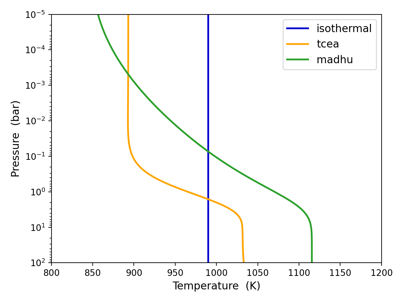
Temperature-profile Examples

Note

Before running this example, download the configuration files shown above, e.g., with these shell commands:

tutorial_path=https://raw.githubusercontent.com/pcubillos/pyratbay/master/examples/tutorial
wget $tutorial_path/pt_isothermal.cfg
wget $tutorial_path/pt_guillot.cfg
wget $tutorial_path/pt_madhu.cfg

The following Python script creates and plots the pressure-temperature profiles for the configuration files shown above:

import matplotlib.pyplot as plt
plt.ion()

import pyratbay as pb
import pyratbay.constants as pc

# Generate PT profiles:
press, t_iso = pb.run("pt_isothermal.cfg")[0:2]
press, t_guillot = pb.run("pt_guillot.cfg")[0:2]
press, t_madhu = pb.run("pt_madhu.cfg")[0:2]

# Plot the PT profiles:
plt.figure(11)
plt.clf()
plt.semilogy(t_iso, press/pc.bar, color='mediumblue', lw=2, label='isothermal')
plt.semilogy(t_guillot, press/pc.bar, color='orange', lw=2, label='guillot')
plt.semilogy(t_madhu, press/pc.bar, color='tab:green', lw=2, label='madhu')
plt.ylim(100, 1e-5)
plt.xlim(800, 1200)
plt.legend(loc="best", fontsize=12)
plt.xlabel("Temperature  (K)", fontsize=12)
plt.ylabel("Pressure  (bar)", fontsize=12)
plt.tight_layout()

And the results should look like this:

Note

If any of the required variables is missing form the configuration file, Pyrat Bay will throw an error indicating the missing value, and stop executing the run. Similarly, Pyrat Bay will throw a warning for a missing variable that was defaulted, and continue executing the run.

Abundance Profiles

Currently, there are two chemistry models (chemistry argument) to compute volume-mixing-ratio abundances: uniform or thermochemical equilibrium. Each one requires a different set of arguments, which is described in the table and sections below:

Models (`chemistry`)	Required arguments [optional arguments]	References
uniform	`species`, `uniform`	—
tea	`species`, `elements`, [`xsolar`, `escale` ]	[Blecic2016]

Uniform abundances

To produce a uniform-abundance model, the configuration file must contain the species key specifying a list of the name of the species to include in the atmosphere, and the uniform key specifying the mole mixing fraction for each of the species listed in species. An atmosphere config file must also set the atmfile key specifying the output atmospheric file name.

Here is an example of a uniform atmosphere configuration file (atmosphere_uniform.cfg):

[pyrat]

# Pyrat Bay run mode, select from: [tli atmosphere spectrum opacity mcmc]
runmode = atmosphere

# Pressure at the top and bottom of the atmosphere, and number of layers:
ptop = 1.0e-6 bar
pbottom = 100.0 bar
nlayers = 100

# Temperature-profile model, select from [isothermal guillot madhu]
tmodel = guillot
# log(kappa') log(g1) log(g2) alpha T_irr  T_int
tpars = -6.0  -0.25   0.0     0.0   950.0  100.0

# Output atmospheric model:
atmfile = WASP-00c.atm

# Chemistry model, select from [uniform tea]
chemistry = uniform
# Atmospheric composition and abundances:
species = H2   He    Na   H2O  CH4  CO   CO2  NH3  HCN  N2
uniform = 0.85 0.149 5e-6 2e-3 1e-4 5e-4 1e-6 1e-5 1e-9 2e-4

# Verbosity level (<0:errors, 0:warnings, 1:headlines, 2:details, 3:debug):
verb = 2

Thermochemical-equilibrium Abundances

Pyrat Bay computes abundances in thermochemical equilibrium via the TEA package [Blecic2016], by minimizing the Gibbs free energy at each layer. To produce a TEA model, the configuration file must contain the species key specifying the species to include in the atmosphere, the elements key specifying the elemental composition. An atmosphere config file must also set the atmfile key specifying the output atmospheric file name.

The TEA run assumes a solar elemental composition from [Asplund2009]; however, the user can scale the abundance of metals by setting the xsolar key, or can scale individual elemental abundances by setting the escale key element and scale factor pairs:

Here is an example of a thermochemical-equilibrium atmosphere configuration file (atmosphere_tea.cfg):

[pyrat]

# Pyrat Bay run mode, select from: [tli atmosphere spectrum opacity mcmc]
runmode = atmosphere

# Pressure at the top and bottom of the atmosphere, and number of layers:
ptop = 1.0e-6 bar
pbottom = 100.0 bar
nlayers = 100

# Temperature-profile model, select from [isothermal guillot madhu]
tmodel = guillot
# log(kappa') log(g1) log(g2) alpha T_irr   T_int
tpars = -6.0  -0.25   0.0     0.0   950.0  100.0

# Output atmospheric model:
atmfile = WASP-00b.atm

# Chemistry model, select from [uniform tea]
chemistry = tea
# Output atmospheric composition:
species = H He C N O Na H2 H2O CH4 CO CO2 NH3 HCN N2

# Set elemental abundance of all metals (dex units, relative to solar):
# (2x solar metallicity for everything except H, He)
metallicity = 0.3

# Scale abundances of specific elements (dex units):
# (Further enhance carbon by 10x and nitrogen by 2x)
e_scale =
    C 1.0
    N 0.3

# Verbosity level (<0:errors, 0:warnings, 1:headlines, 2:details, 3:debug):
verb = 2

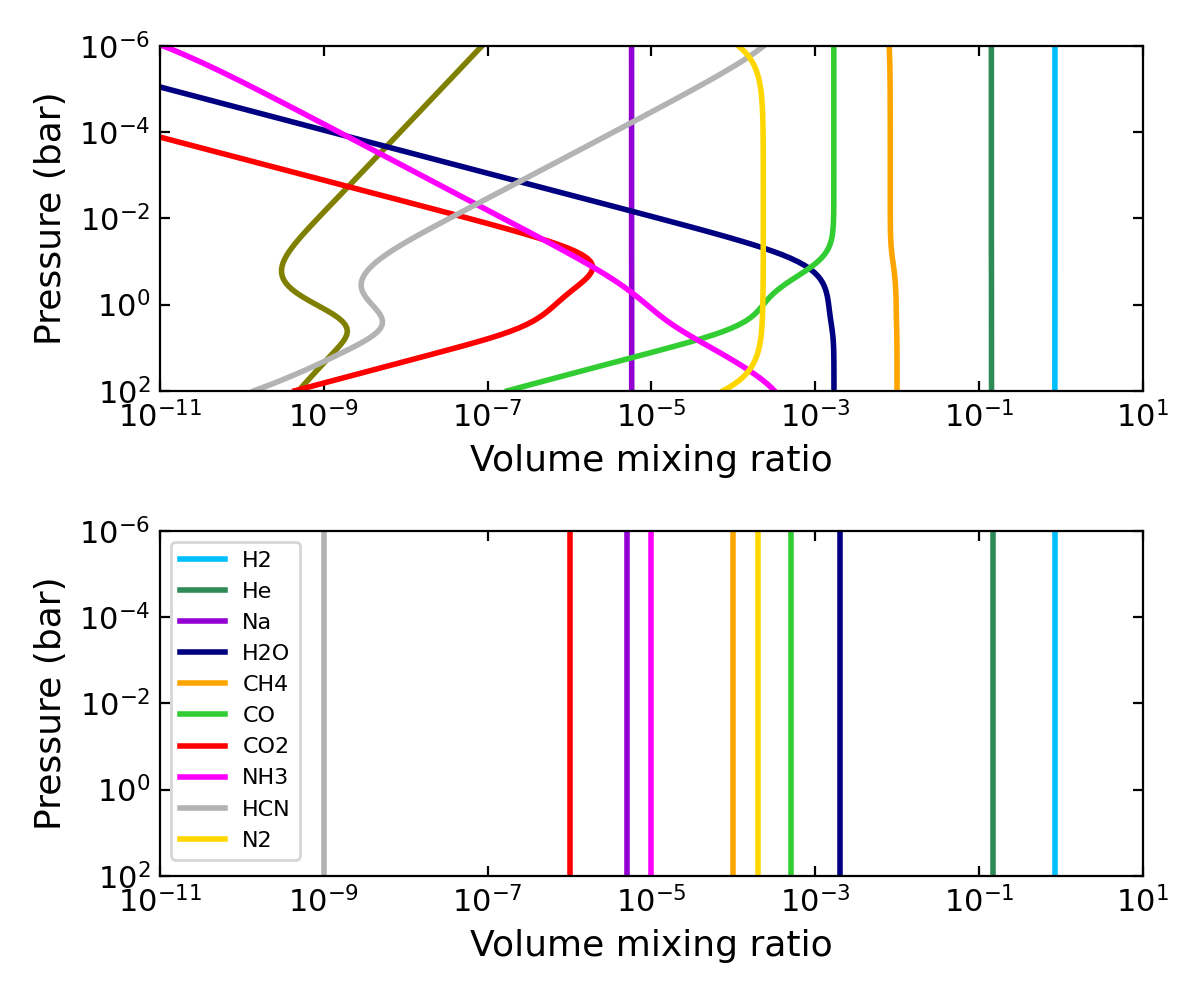
Abundance-profile Examples

Note

Before running this example, download the configuration files shown above, e.g., with these shell commands:

tutorial_path=https://raw.githubusercontent.com/pcubillos/pyratbay/master/examples/tutorial
wget $tutorial_path/atmosphere_tea.cfg
wget $tutorial_path/atmosphere_uniform.cfg

The following Python script creates and plots the abundance Aprofiles for the configuration files shown above:

import matplotlib.pyplot as plt
plt.ion()

import pyratbay as pb
import pyratbay.plots as pp

# Generate a uniform and a thermochemical-equilibrium atmospheric model:
pressure, temp, vmr_tea, species_tea, radius = pb.run("atmosphere_tea.cfg")
pressure, temp, vmr_uni, species_uni, radius = pb.run("atmosphere_uniform.cfg")

# Plot the results:
plt.figure(12, (6,5))
plt.clf()
ax = plt.subplot(211)
ax1 = pp.abundance(
    vmr_tea, pressure, species_tea,
    colors='default', xlim=[1e-11, 10.0], legend_fs=0, ax=ax,
)
ax = plt.subplot(212)
ax2 = pp.abundance(
    vmr_uni, pressure, species_uni,
    colors='default', xlim=[1e-11, 10.0], legend_fs=8, ax=ax,
)
plt.tight_layout()

And the results should look like this:

Altitude Profiles

If the user sets the radmodel key, the code will to compute the atmospheric altitude profile (radius profile). The currently available models solve for the hydrostatic-equilibrium equation, combined with the ideal gas law with a pressure-dependent gravity (radmodel=hydro_m, recommended):

\[\frac{dr}{r^2} = -\frac{k_{\rm B}T}{\mu G M_p} \frac{dp}{p},\]

or a constant surface gravity (radmodel=hydro_g):

\[dr = -\frac{k_{\rm B}T}{\mu g} \frac{dp}{p},\]

where \(M_{\rm p}\) is the mass of the planet, \(T(p)\) is the atmospheric temperature, \(\mu(p)\) is the atmospheric mean molecular mass, \(k_{\rm B}\) is the Boltzmann constant, and \(G\) is the gravitational constant. Note that \(T(p)\) and \(\mu(p)\) are computed from the models of the Temperature Profiles and Abundance Profiles, respectively.

To obtain the particular solution of these differential equations, the user needs to supply a pair of radius–pressure reference values to define the boundary condition \(r(p_0) = R_0\). The rplanet and refpressure keys set \(R_0\) and \(p_0\), respectively. The mplanet and gplanet keys set the planetary mass (\(M_p\)) and surface gravity (\(g\)), respectively.

Note

Note that the user needs only to define two out of the three \(\{R_0, M_p, g\}\) variables, since they are related through the equation: \(g(R_0) = G M_p / R_0^2\).

Note that the selection of the \(\{p_0,R_0\}\) pair is arbitrary. A good practice is to choose values close to the transit radius of the planet. Although the pressure at the transit radius is a priori unknown for a give particular case [Griffith2014], its value lies at around 0.1 bar.

Here is an example of a hydrostatic-equilibrium atmosphere configuration file (atmosphere_hydro_m.cfg):

[pyrat]

# Pyrat Bay run mode, select from: [tli atmosphere spectrum opacity mcmc]
runmode = atmosphere

# Pressure at the top and bottom of the atmosphere, and number of layers:
ptop = 1.0e-6 bar
pbottom = 100.0 bar
nlayers = 100

# Temperature-profile model, select from [isothermal guillot madhu]
tmodel = guillot
# log(kappa') log(g1) log(g2) alpha T_irr  T_int
tpars = -6.0  -0.25   0.0     0.0   950.0  100.0

# Output atmospheric model:
atmfile = WASP-00c.atm

# Chemistry model, select from [uniform tea]
chemistry = uniform
# Atmospheric composition and abundances:
species = H2   He    Na   H2O  CH4  CO   CO2  NH3  HCN  N2
uniform = 0.85 0.149 5e-6 2e-3 1e-4 5e-4 1e-6 1e-5 1e-9 2e-4

# Altitude/radius profile model, select from [hydro_m, hydro_g]:
radmodel = hydro_m
rplanet = 2.87 rearth
mplanet = 2.86 mearth
refpressure = 0.1 bar

# Verbosity level (<0:errors, 0:warnings, 1:headlines, 2:details, 3:debug):
verb = 2

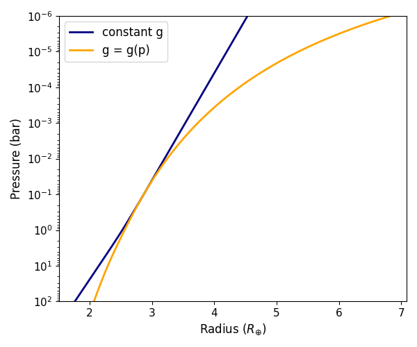
Altitude-profile Examples

Note

Before running this example, download the configuration files shown above, e.g., with these shell commands:

tutorial_path=https://raw.githubusercontent.com/pcubillos/pyratbay/master/examples/tutorial
wget $tutorial_path/atmosphere_hydro_m.cfg
wget $tutorial_path/atmosphere_hydro_g.cfg

The following Python script creates and plots the profiles for the configuration file shown above:

import matplotlib.pyplot as plt
plt.ion()

import pyratbay as pb
import pyratbay.constants as pc

# Kepler-11c mass and radius:
pressure, temp, q, species, radius = pb.run("atmosphere_hydro_m.cfg")
pressure, temp, q, species, radius_g = pb.run("atmosphere_hydro_g.cfg")

# Plot the results:
plt.figure(12, (6,5))
plt.clf()
ax = plt.subplot(111)
ax.semilogy(radius_g/pc.rearth, pressure/pc.bar, lw=2, c='navy', label='constant g')
ax.semilogy(radius/pc.rearth, pressure/pc.bar, lw=2, c='orange', label='g = g(p)')
ax.set_ylim(1e2, 1e-6)
ax.set_xlabel(r'Radius $(R_{\oplus})$', fontsize=12)
ax.set_ylabel('Pressure (bar)', fontsize=12)
ax.tick_params(labelsize=11)
ax.legend(loc='upper left', fontsize=12)
plt.tight_layout()

And the results should look like this: